Building Blocks for Hierarchical Nonlinear Factor Analysis

Hierarchical latent variable models can be constructed from simple building blocks. The basic idea is that adapting can be done locally. This provides a way to construct complicated models that can still be used with linear complexity. The formulas and implementation can be done for each block separately therefore reducing the possibility of errors and allowing more attention to other matters. It also increases the extensibility. In this chapter, the building blocks and equations for computation with them are introduced. 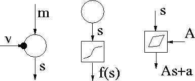The building blocks consist of variable nodes and computation nodes. The symbols for them are shown in Figure .

  

Figure: Left: A Gaussian latent variable s, marked with a circle, has a prior mean m and a prior variance $\exp(-v)$. Middle: A nonlinearity f is applied immediately after a Gaussian variable. Right: An affine transformation is made to the signal vector s.

The network is described using terms of neural networks [24] and Bayesian networks [33] when applicable. The nodes are attached to each other using signals. Each node has input and output values or signals. For variable nodes, input is a value which is used for the prior distribution and output is the value of the variable. The variable nodes are continuous valued with a Gaussian prior. Each variable can be either observed or latent. Time dependent latent variables are called sources or neurons and time independent latent variables are called parameters or weights. For computation nodes, output is a fixed function of the inputs.

Since the variable nodes are probabilistic, the values propagated between the nodes have distributions. When ensemble learning together with a factorial posterior approximation is used, the cost function can be computed by propagating certain expected values instead of full distributions as can be seen in (). Consequently the cost function can be minimised based on gradients w.r.t. these expectations computed by back-propagation [24]. The gradients define the likelihood. Prior probabilities propagate forward, likelihoods propagate backward and they are combined to posterior probabilities.

The input for prior mean of a Gaussian node requires the mean $\left< \cdot \right>$ and variance $\mathrm{Var}\left\{\cdot\right\}$. With a suitable parametrisation, mean $\left< \cdot \right>$ and expected exponential $\left< \exp\cdot \right>$ are required from the input for prior variance. The output of a Gaussian node can provide the mean $\left< \cdot \right>$, variance $\mathrm{Var}\left\{\cdot\right\}$ and expected exponential $\left< \exp\cdot \right>$ and can thus be used as an input to both the mean and variance of another Gaussian node. The expectations required by the inputs and provided by the outputs of different nodes are listed below:

	$\left< \cdot \right>$	$\mathrm{Var}\left\{\cdot\right\}$	$\left< \exp\cdot \right>$
Output provides:
Gaussian	+	+	+
Gaussian with nonlinearity	+	+
addition	+	+	+
multiplication	+	+
Prior for variable nodes requires:
mean of Gaussians	+	+
variance of Gaussians	+		+

The variables can be gathered to vectors and matrices in a straigthforward manner. Other nodes that are compatible with the ones shown here can be found in [66].