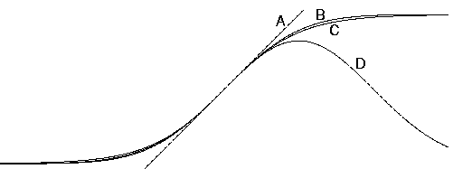
Figure ![[*]](cross_ref_motif.gif) shows some possible transfer
functions. A good nonlinearity should have an area that is close to
linear and another that is saturated. Linear part guarantees the
possibility to use the unit as a linear one. Saturated area makes
sparse representation possible as was seen in
Section . When the input fluctuates inside the the
saturated area, the output does not effectively vary. Thus, the input
does not always need to be precisely determined for the output to be
precise. A nonlinearity with two flat parts can be used as a binary
unit that has two typical output values and almost nothing in between.
shows some possible transfer
functions. A good nonlinearity should have an area that is close to
linear and another that is saturated. Linear part guarantees the
possibility to use the unit as a linear one. Saturated area makes
sparse representation possible as was seen in
Section . When the input fluctuates inside the the
saturated area, the output does not effectively vary. Thus, the input
does not always need to be precisely determined for the output to be
precise. A nonlinearity with two flat parts can be used as a binary
unit that has two typical output values and almost nothing in between.
 |
Some expected values after the nonlinearity can be evaluated for
Gaussian input [20]. Therefore we restrict the
nonlinearity to follow immediately after a Gaussian variable node.
Now the mean, variance and the expected exponential of the output of a
nonlinearity have integral expressions. For most nonlinear functions
it is impossible to compute them analytically, but for the function
![]() the mean and variance do have analytical
expressions. Therefore it is used in this work. The required
expectations of the outputs are
the mean and variance do have analytical
expressions. Therefore it is used in this work. The required
expectations of the outputs are
Gaussian radial basis functions (RBF) [24] use the same
nonlinearity but the input is the distance from a certain point in the
source space rather than one of the sources directly. Ghahramani and
Roweis [20] used Gaussian RBF approximators with
EM algorithm to model nonlinear dynamical systems. They found that
using the Gaussian nonlinearity the integrals become tractable.
Another potential possibility would be to use the error function
![]() ,
since the mean can be evaluated
analytically and the variance can be approximated from above
[15]. This is useful, since increasing the variance increases also
the cost function and minimising an upper bound for the cost
guarantees it to be low. Murphy [50] used the logistic
function approximated iteratively with a Gaussian. Valpola
[62] approximated the same function with a
truncated Taylor series.
,
since the mean can be evaluated
analytically and the variance can be approximated from above
[15]. This is useful, since increasing the variance increases also
the cost function and minimising an upper bound for the cost
guarantees it to be low. Murphy [50] used the logistic
function approximated iteratively with a Gaussian. Valpola
[62] approximated the same function with a
truncated Taylor series.
Hornik [26] and Funahashi [17] have
independently shown that MLP networks are universal approximators,
that is, given enough hidden units the mapping from inputs to outputs
can approximate any measurable function to any desired degree of
accuracy. This result was proven for any non-decreasing nonlinearity
f(s) that has the limits
![]() and
and
![]() .
Unfortunately, that is not true
for the function
.
Unfortunately, that is not true
for the function
![]() .
Future work might include a
comparison with other nonlinearities and perhaps the property of
universal approximation could be proven at least for a finite
interval.
.
Future work might include a
comparison with other nonlinearities and perhaps the property of
universal approximation could be proven at least for a finite
interval.