Missing values in speech spectra

In hierarchical nonlinear factor analysis (HNFA) Valpola03ICA_Nonlin, there are a number of layers of Gaussian variables, the bottom-most layer corresponding to the data. There is a nonlinearity and a linear mixture mapping from each layer to all the layers below it.

HNFA resembles the model structure in Section 5.3. The model structure is depicted in the left subfigure of Fig. 12. Model equations are

$${\mathbf{h}}(t) = {\mathbf{A}}{\mathbf{s}}(t) + {\mathbf{a}} + {\mathbf{n}}_h(t)$$ (51)

$${\mathbf{x}}(t) = {\mathbf{B}}\boldsymbol{\phi}[ {\mathbf{h}}(t) ] + {\mathbf{C}}{\mathbf{s}}(t) + {\mathbf{b}} + {\mathbf{n}}_x(t) \, ,$$ (52)

where ${\mathbf{n}}_h(t)$ and ${\mathbf{n}}_x(t)$ are Gaussian noise terms and the nonlinearity $\phi(\xi) = \exp(-\xi^2)$ again operates on each element of its argument vector separately. Note that we have included a short-cut mapping ${\mathbf{C}}$ from sources to observations. This means that hidden nodes only need to model the deviations from linearity.

HNFA is compared against three other methods. Factor analysis (FA) is a linear method described in Section 5.2. It is a special case of HNFA where the dimensionality of ${\mathbf{h}}(t)$ is zero. Nonlinear factor analysis (NFA) Lappalainen00, Honkela05NIPS differs from HNFA in that it does not use mediating variables ${\mathbf{h}}(t)$:

$${\mathbf{x}}(t) = {\mathbf{B}}\tanh[ {\mathbf{A}}{\mathbf{s}}(t) + {\mathbf{a}}] + {\mathbf{b}} + {\mathbf{n}}_x(t).$$ (53)

Note that NFA has multiple computational paths between ${\mathbf{s}}(t)$ and ${\mathbf{x}}(t)$, which leads to a higher computational complexity compared to HNFA.

The self-organising map SOM Kohonen01 differs most from the other methods. A rectangular map has a number of map units with associated model vectors that are points in the data space. Each data point is matched to the closest map unit. The model vectors of the best-matching unit and its neighbours in the map are moved slightly towards the data point. See Kohonen01, Haykin98 for details.

Figure 12: Left: The model structure for hierarchical nonlinear factor analysis (HNFA). Right: Some speech data with and without missing values (Setting 1) and the reconstruction given by HNFA.

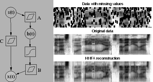The data set consisted of speech spectrograms from several Finnish subjects. Short term spectra were windowed to 30 dimensions with a standard preprocessing procedure for speech recognition. It is clear that a dynamic source model would give better reconstructions, but in this case the temporal information was left out to ease the comparison of the models. Half of the about 5000 samples were used as test data with some missing values. Missing values were set in four different ways to measure different properties of the algorithms (Figure 13):

1. 38 percent of the values are set to miss randomly in $4 \times 4$ patches. (Right subfigure of Figure 12)
   
2. Training and testing sets are randomly permuted before setting missing values in $4 \times 4$ patches as in Setting 1.
   
3. 10 percent of the values are set to miss randomly independent of any neighbours. This is an easier setting, since simple smoothing using nearby values would give fine reconstructions.
   
4. Training and testing sets are permuted and 10 percent of the values are set to miss independently of any neighbours.
   

Figure 13: Four different experimental settings with the speech data used for measuring different properties of the algorithms.

We tried to optimise each method and in the following, we describe how we got the best results. The self-organising map was run using the SOM Toolbox Vesanto99somtoolbox with long learning time, 2500 map units and random initialisations. In other methods, the optimisation was based on minimising the cost function or its approximation. NFA was learned for 5000 sweeps through data using a Matlab implementation. Varying number of sources were tried out and the best ones were used as the result. The optimal number of sources was around 12 to 15 and the size used for the hidden layer was 30. A large enough number should do, since the algorithm can effectively prune out parts that are not needed.

In factor analysis (FA), the number of sources was 28. In hierarchical nonlinear factor analysis (HNFA), the number of sources at the top layer was varied and the best runs according to the cost function were selected. In those runs, the size of the top layer varied from 6 to 12 and the size of the middle layer, which is determined during learning, turned out to vary from 12 to 30. HNFA was run for 5000 sweeps through data. Each experiment with NFA or HNFA took about 8 hours of processor time, while FA and SOM were faster.

Several runs were conducted with different random initialisations but with the same data and the same missing value pattern for each setting and for each method. The number of runs in each cell is about 30 for HNFA, 4 for NFA and 20 for the SOM. FA always converges to the same solution. The mean and the standard deviation of the mean square reconstruction error are:

	FA	HNFA	NFA	SOM
Setting 1	$1.87$	$1.80 \pm 0.03$	$1.74 \pm 0.02$	$1.69 \pm 0.02$
Setting 2	$1.85$	$1.78 \pm 0.03$	$1.71 \pm 0.01$	$1.55 \pm 0.01$
Setting 3	$0.57$	$0.55 \pm .005$	$0.56 \pm .002$	$0.86 \pm 0.01$
Setting 4	$0.58$	$0.55 \pm .008$	$0.58 \pm .004$	$0.87 \pm 0.01$

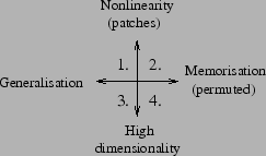
The order of results of the Setting 1 follow our expectations on the nonlinearity of the models. The SOM with highest nonlinearity gives the best reconstructions, while NFA, HNFA and finally FA follow in that order. The results of HNFA vary the most - there is potential to develop better learning schemes to find better solutions more often. The sources ${\mathbf{h}}(t)$ of the hidden layer did not only emulate computation nodes, but they were also active themselves. Avoiding this situation during learning could help to find more nonlinear and thus perhaps better solutions.

In the Setting 2, due to the permutation, the test set contains vectors very similar to some in the training set. Therefore, generalisation is not as important as in the Setting 1. The SOM is able to memorise details corresponding to individual samples better due to its high number of parameters. Compared to the Setting 1, SOM benefits a lot and makes clearly the best reconstructions, while the others benefit only marginally.

The Settings 3 and 4, which require accurate expressive power in high dimensionality, turned out not to differ from each other much. The basic SOM has only two intrinsic dimensions⁴ and therefore it was clearly poorer in accuracy. Nonlinear effects were not important in these settings, since HNFA and NFA were only marginally better than FA. HNFA was better than NFA perhaps because it had more latent variables when counting both ${\mathbf{s}}(t)$ and ${\mathbf{h}}(t)$.

To conclude, HNFA lies between FA and NFA in performance. HNFA is applicable to high dimensional problems and the middle layer can model part of the nonlinearity without increasing the computational complexity dramatically. FA is better than SOM when expressivity in high dimensions is important, but SOM is better when nonlinear effects are more important. The extensions of FA, NFA and HNFA, expectedly performed better than FA in each setting. It may be possible to enhance the performance of NFA and HNFA by new learning schemes whereas especially FA is already at its limits. On the other hand, FA is best if low computational complexity is the determining factor.