A hierarchical variance model

Figure 6 (right subfigure) presents a hierarchical model for the variance, and also shows how it can be constructed by first learning simpler structures shown in the left and middle subfigures of Fig. 6. This is necessary, because learning a hierarchical model having different types of nodes from scratch in a completely unsupervised manner would be too demanding a task, ending quite probably into an unsatisfactory local minimum.

The final rightmost variance model in Fig. 6 is somewhat involved in that it contains both nonlinearities and hierarchical modelling of variances. Before going into its mathematical details and into the two simpler models in Fig. 6, we point out that we have considered in our earlier papers related but simpler block models. In Valpola03ICA_Nonlin, a hierarchical nonlinear model for the data ${\bf x}(t)$ is discussed without modelling the variance. Such a model can be applied for example to nonlinear ICA or blind source separation. Experimental results Valpola03ICA_Nonlin show that this block model performs adequately in the nonlinear BSS problem, even though the results are slightly poorer than for our earlier computationally more demanding model Lappalainen00,Valpola03IEICE,Honkela05NIPS with multiple computational paths.

In another paper Valpola04SigProc, we have considered hierarchical modelling of variance using the block approach without nonlinearities. Experimental results on biomedical MEG (magnetoencephalography) data demonstrate the usefulness of hierarchical modelling of variances and existence of variance sources in real-world data.

Figure 6: Construction of a hierarchical variance model in stages from simpler models. Left: In the beginning, a variance source is attached to each Gaussian observation node. The nodes represent vectors. Middle: A layer of sources with variance sources attached to them is added. They layers are connected through a nonlinearity and an affine mapping. Right: Another layer is added on the top to form the final hierarchical variance model.

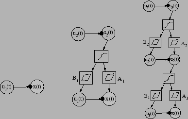Learning starts from the simple structure shown in the left subfigure of Fig. 6. There a variance source is attached to each Gaussian observation node. The nodes represent vectors, with ${\bf u}_1(t)$ being the output vector of the variance source and ${\bf x}(t)$ the $t^$th observation (data) vector. The vectors ${\bf u}_1(t)$ and ${\bf x}(t)$ have the same dimension, and each component of the variance vector ${\bf u}_1(t)$ models the variance of the respective component of the observation vector ${\bf x}(t)$.

Mathematically, this simple first model obeys the equations

$${\bf x}(t) = {\bf a}_1 + {\bf n}_x(t)$$ (33)

$${\bf u}_1(t) = {\bf b}_1 + {\bf n}_{u_1}(t)$$ (34)

Here the vectors ${\bf a}_1$ and ${\bf b}_1$ denote the constant means (bias terms) of the data vector ${\bf x}(t)$ and the variance variable vector ${\bf u}_1(t)$, respectively. The additive ``noise'' vector ${\bf n}_x(t)$ determines the variances of the components of ${\bf x}(t)$. It has a Gaussian distribution with a zero mean and variance $\exp [-{\bf u}_1(t)]$:

$${\bf n}_x(t) \sim \mathcal N({\bf0},\exp[ -{\bf u}_1(t) ])$$ (35)

More precisely, the shorthand notation $\mathcal N({\bf0},\exp [ -{\bf u}_1(t)] )$ means that each component of ${\bf n}_x(t)$ is Gaussian distributed with a zero mean and variance defined by the respective component of the vector $\exp [-{\bf u}_1(t)]$. The exponential function $\exp(\cdot)$ is applied separately to each component of the vector $-{\bf u}_1(t)$. Similarly,

$${\bf n}_{u_1}(t) \sim \mathcal N({\bf0},\exp \left[-{\bf v}_1 \right])$$ (36)

where the components of the vector ${\bf v}_1$ define the variances of the zero mean Gaussian variables ${\bf n}_{u_1}(t)$.

Consider then the intermediate model shown in the middle subfigure of Fig. 6. In this second learning stage, a layer of sources with variance sources attached to them is added. These sources are represented by the source vector ${\bf s}_2(t)$, and their variances are given by the respective components of the variance vector ${\bf u}_2(t)$ quite similarly as in the left subfigure. The (vector) node between the source vector ${\bf s}_2(t)$ and the variance vector ${\bf u}_1(t)$ represents an affine transformation with a transformation matrix ${\mathbf{A}}_{1}$ including a bias term. Hence the prior mean inputted to the Gaussian variance source having the output ${\bf u}_1(t)$ is of the form ${\bf B}_1 {\bf f}({\bf s}_2(t)) + {\bf b}_1$, where ${\bf b}_1$ is the bias vector, and ${\bf f}(\cdot)$ is a vector of componentwise nonlinear functions (9). Quite similarly, the vector node between ${\bf s}_2(t)$ and the observation vector ${\bf x}(t)$ yields as its output the affine transformation ${\bf A}_1{\bf f}({\bf s}_2(t)) + {\bf a}_1$, where ${\bf a}_1$ is a bias vector. This in turn provides the input prior mean to the Gaussian node modelling the observation vector ${\bf x}(t)$.

The mathematical equations corresponding to the model represented graphically in the middle subfigure of Fig. 6 are:

$${\bf x}(t) = {\bf A}_1 {\bf f}({\bf s}_2(t)) + {\bf a}_1 + {\bf n}_x(t)$$ (37)

$${\bf u}_1(t) = {\bf B}_1 {\bf f}({\bf s}_2(t)) + {\bf b}_1 + {\bf n}_{u_1}(t)$$ (38)

$${\bf s}_2(t) = {\bf a}_2 + {\bf n}_{s_2}(t)$$ (39)

$${\bf u}_2(t) = {\bf b}_2 + {\bf n}_{u_2}(t)$$ (40)

Compared with the simplest model (33)-(34), one can observe that the source vector ${\bf s}_2(t)$ of the second (upper) layer and the associated variance vector ${\bf u}_2(t)$ are of quite similar form, given in Eqs. (39)-(40). The models (37)-(38) of the data vector ${\bf x}(t)$ and the associated variance vector ${\bf u}_1(t)$ in the first (bottom) layer differ from the simple first model (33)-(34) in that they contain additional terms ${\bf A}_1 {\bf f}({\bf s}_2(t))$ and ${\bf B}_1 {\bf f}({\bf s}_2(t))$, respectively. In these terms, the nonlinear transformation ${\bf f}({\bf s}_2(t))$ of the source vector ${\bf s}_2(t)$ coming from the upper layer have been multiplied by the linear mixing matrices ${\bf A}_1$ and ${\bf B}_1$. All the ``noise'' terms ${\bf n}_x(t)$, ${\bf n}_{u_1}(t)$, ${\bf n}_{s_2}(t)$, and ${\bf n}_{u_2}(t)$ in Eqs. (37)-(40) are modelled by similar zero mean Gaussian distributions as in Eqs. (35) and (36).

In the last stage of learning, another layer is added on the top of the network shown in the middle subfigure of Fig. 6. The resulting structure is shown in the right subfigure. The added new layer is quite similar as the layer added in the second stage. The prior variances represented by the vector ${\bf u}_3(t)$ model the source vector ${\bf s}_3(t)$, which is turn affects via the affine transformation ${\bf B}_2{\bf f}({\bf s}_3(t)) + {\bf b}_2$ to the mean of the mediating variance node ${\bf u}_2(t)$. The source vector ${\bf s}_3(t)$ provides also the prior mean of the source ${\bf s}_2(t)$ via the affine transformation ${\bf A}_2{\bf f}({\bf s}_3(t)) + {\bf a}_2$.

The model equations (37)-(38) for the data vector ${\bf x}(t)$ and its associated variance vector ${\bf u}_1(t)$ remain the same as in the intermediate model shown graphically in the middle subfigure of Fig. 6. The model equations of the second and third layer sources ${\bf s}_2(t)$ and ${\bf s}_3(t)$ as well as their respective variance vectors ${\bf u}_2(t)$ and ${\bf u}_3(t)$ in the rightmost subfigure of Fig. 6 are given by

$${\bf s}_2(t) = {\bf A}_2 {\bf f}({\bf s}_3(t)) + {\bf a}_2 + {\bf n}_{s_2}(t)$$ (41)

$${\bf u}_2(t) = {\bf B}_2 {\bf f}({\bf s}_3(t)) + {\bf b}_2 + {\bf n}_{u_2}(t)$$ (42)

$${\bf s}_3(t) = {\bf a}_3 + {\bf n}_{s_3}(t)$$ (43)

$${\bf u}_3(t) = {\bf b}_3 + {\bf n}_{u_3}(t)$$ (44)

Again, the vectors ${\bf a}_2$, ${\bf b}_2$, ${\bf a}_3$, and ${\bf b}_3$ represent the constant means (biases) in their respective models, and ${\bf A}_2$ and ${\bf B}_2$ are mixing matrices with matching dimensions. The vectors ${\bf n}_{s_2}(t)$, ${\bf n}_{u_2}(t)$, ${\bf n}_{s_3}(t)$, and ${\bf n}_{u_3}(t)$ have similar zero mean Gaussian distributions as in Eqs. (35) and (36).

It should be noted that in the resulting network the number of scalar-valued nodes (size of the layers) can be different for different layers. Additional layers could be appended in the same manner. The final network of the right subfigure in Fig. 6 utilises variance nodes in building a hierarchical model for both the means and variances. Without the variance sources the model would correspond to a nonlinear model with latent variables in the hidden layer. As already mentioned, we have considered such a nonlinear hierarchical model in Valpola03ICA_Nonlin. Note that computation nodes as hidden nodes would result in multiple paths from the latent variables of the upper layer to the observations. This type of structure was used in Lappalainen00, and it has a quadratic computational complexity as opposed to linear one of the networks in Figure 6.