In this section an experiment with a dynamical model for variances applied to image sequence analysis is reported. The motivation behind modelling variances is that in many natural signals, there exists higher order dependencies which are well characterised by correlated variances of the signals Parra00NIPS. Hence we postulate that we should be able to better catch the dynamics of a video sequence by modelling the variances of the features instead of the features themselves. This indeed is the case as will be shown.
The model considered can be summarised by the following set of equations:
The sparsity of ![]() is crucial as the computational
complexity of the learning algorithm depends on the number
of connections from
is crucial as the computational
complexity of the learning algorithm depends on the number
of connections from
![]() to
to
![]() . The same goal could
have been reached with a different kind of approach as well. Instead
of constraining the mapping to be sparse from the very beginning
of learning it could have been allowed to be full for a number
of iterations and only after that pruned based on the cost function
as explained in Section 6.2. But as the basis
for image sequences tends to get sparse anyway, it is a waste
of computational resources to wait while most of the weights
in the linear mapping tend to zero.
. The same goal could
have been reached with a different kind of approach as well. Instead
of constraining the mapping to be sparse from the very beginning
of learning it could have been allowed to be full for a number
of iterations and only after that pruned based on the cost function
as explained in Section 6.2. But as the basis
for image sequences tends to get sparse anyway, it is a waste
of computational resources to wait while most of the weights
in the linear mapping tend to zero.
For comparison purposes, we postulate another model where the dynamical relations are sought directly between the sources leading to the following model equations:
The data
![]() was a video image sequence Hateren98 of dimensions
was a video image sequence Hateren98 of dimensions
![]() . That is, the data consisted of 4000
subsequent digital images of the size
. That is, the data consisted of 4000
subsequent digital images of the size
![]() . A part
of the data set is shown in Figure 14.
. A part
of the data set is shown in Figure 14.
Both models were learned by iterating the learning algorithm
2000 times at which stage a sufficient convergence was attained.
The first hint of the superiority of the DynVar model was provided
by the difference of the cost between the models which was 28 bits/frame
[for the coding interpretation, see][]Honkela04TNN. To further
evaluate the performance
of the models, we considered a simple prediction task where the next
frame was predicted based on the previous ones.
The predictive distributions,
![]() ,
for the models can be approximately computed based on the posterior
approximation.
The means of the predictive distributions are very similar for both
of the models. Figure 15 shows the means of the DynVar
model for the same sequence as in Figure 14.
The means themselves are not very interesting, since they mainly
reflect the situation in the previous frame.
However, the DynVar model provides also a rich
model for the variances. The standard deviations of its predictive
distribution are shown in Figure 16. White stands for a large
variance and black for a small one. Clearly, the model
is able to increase the predicted variance in the area of high
motion activity and hence provide better predictions. We can offer
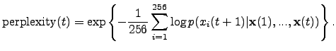
quantitative support for this claim by computing the predictive perplexities
for the models. Predictive perplexity is widely used in language modelling
and it is defined as
,
for the models can be approximately computed based on the posterior
approximation.
The means of the predictive distributions are very similar for both
of the models. Figure 15 shows the means of the DynVar
model for the same sequence as in Figure 14.
The means themselves are not very interesting, since they mainly
reflect the situation in the previous frame.
However, the DynVar model provides also a rich
model for the variances. The standard deviations of its predictive
distribution are shown in Figure 16. White stands for a large
variance and black for a small one. Clearly, the model
is able to increase the predicted variance in the area of high
motion activity and hence provide better predictions. We can offer
quantitative support for this claim by computing the predictive perplexities
for the models. Predictive perplexity is widely used in language modelling
and it is defined as
 |
|
[width=0.5]VarPredVar
|
The possible applications for a model of image sequences include video compression, motion detection, early stages of computer vision, and making hypotheses on biological vision.