We could go on formulating reconstruction mappings and solving the
output mappings, but this would become increasingly difficult.
Moreover, it is not at all clear that we would get a network which
would have the kind of competition behaviour we sketched in the
beginning of this section. Figure 3.3 shows an example
where the simple linear reconstruction does not yield a sparse code.
The weight vector ![]() is much closer to the input than the
two other weight vectors, but according to a linear reconstruction it
would not be used in the representation. This is due to the fact that
linear reconstruction does not promote sparsity in any way. If we use
linear reconstruction and find the optimal outputs using
equation 2.1, we obtain a dense code, because the
reconstruction error is minimised when all the neurons are allowed to
participate in the representation of the input. We need constraints
for the outputs which assure the sparsity of the representation.
is much closer to the input than the
two other weight vectors, but according to a linear reconstruction it
would not be used in the representation. This is due to the fact that
linear reconstruction does not promote sparsity in any way. If we use
linear reconstruction and find the optimal outputs using
equation 2.1, we obtain a dense code, because the
reconstruction error is minimised when all the neurons are allowed to
participate in the representation of the input. We need constraints
for the outputs which assure the sparsity of the representation.
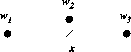
Figure 3.3:
An example of a situation where the reconstruction error
minimisation does not yield a sparse code. All vectors are
supposed to be nearly parallel and 3-dimensional. The figure
shows a view from top (cf. a map of a small area on globe). The
reconstruction is optimal when neurons 1 and 3 represent the
input. However, the code would be more sparse if the neuron 2
represented the input.
It should be reminded that we are using reconstruction error minimisation only because it allows easy derivation for algorithms and assures that the representation generated by the network contains information about the input. Our ultimate goal is not to find an exact reconstruction mapping, but to find a mapping which can generate sparse codes. If we can find outputs that approximately minimise the reconstruction error in equation 2.1, we can use the result in equation 2.2 to derive the learning rule and even an approximate minimisation will ensure that the outputs contain information about the inputs.
We shall now leave the reconstruction mapping for a moment and
consider a way to formulate the constraints for the outputs. We have
already found out that the winning strengths in
equation 3.5 are able to measure the competition between
two neurons. If we have more than two neurons we can still measure
the competition between each pair of neurons and try to combine these
competitions to a final winning strength. By combining equations
3.4 and 3.5 we can define a winning ratio
![]() between each pair of neurons i and j:
between each pair of neurons i and j:
where ![]() and
and ![]() . If there were only two neurons in the
network we could write
. If there were only two neurons in the
network we could write ![]() and we would get the same
solution as in equation 3.5. When we have more than two
neurons we need a way to combine the winning ratios in order to obtain
the winning strengths
and we would get the same
solution as in equation 3.5. When we have more than two
neurons we need a way to combine the winning ratios in order to obtain
the winning strengths ![]() .
.
One can think that the winning ratios ![]() are fuzzy truth
values
are fuzzy truth
values for propositions ``Neuron i is a winner when it
competes with neuron j''. This suggests the use of some kind of
fuzzy and-operation to combine the winning ratios: neuron i is a
winner if it wins the competition with neuron 1 and 2 and
for propositions ``Neuron i is a winner when it
competes with neuron j''. This suggests the use of some kind of
fuzzy and-operation to combine the winning ratios: neuron i is a
winner if it wins the competition with neuron 1 and 2 and ![]() and
n. A simple choice for and-operation is the product of truth
values. We could simply calculate the product of
and
n. A simple choice for and-operation is the product of truth
values. We could simply calculate the product of ![]() over index
j to obtain the winning strengths for neuron i.
over index
j to obtain the winning strengths for neuron i.
However, there would be a small problem. Suppose that neuron 1 has
lost the competition with neuron 2, that is, ![]() . It follows
that
. It follows
that ![]() . This is reasonable, since the neuron cannot be a
winner if it has totally lost in competition with another neuron. The
problem is that
. This is reasonable, since the neuron cannot be a
winner if it has totally lost in competition with another neuron. The
problem is that ![]() for other neurons than 2 may differ from one.
This means that other neurons are competing with a neuron that has
already lost. Since the lost neuron does not convey any information
it would be reasonable that it would not affect the outputs of other
neurons. This can be fixed by weighing the winning ratios
for other neurons than 2 may differ from one.
This means that other neurons are competing with a neuron that has
already lost. Since the lost neuron does not convey any information
it would be reasonable that it would not affect the outputs of other
neurons. This can be fixed by weighing the winning ratios ![]() in
the product by the winning strengths. We can now examine the
solutions to the preliminary winning strengths
in
the product by the winning strengths. We can now examine the
solutions to the preliminary winning strengths ![]() in the
following equation:
in the
following equation:
We have named the values ![]() preliminary winning strengths, since
they do not necessarily satisfy the property
preliminary winning strengths, since
they do not necessarily satisfy the property ![]() , but we
can use
, but we
can use ![]() to compute values
to compute values ![]() which do satisfy it, as will
be shown later on. The weights are put to the exponent, because we
are dealing with a product of numbers. We have also introduced a
parameter
which do satisfy it, as will
be shown later on. The weights are put to the exponent, because we
are dealing with a product of numbers. We have also introduced a
parameter ![]() which can be used to control the amount of
competition.
which can be used to control the amount of
competition.
The preliminary winning strengths ![]() appear in both sides of
equation 3.7 and it is impossible to find a solution in a
closed form. However, this time we can prune most of the neurons from
the computation of
appear in both sides of
equation 3.7 and it is impossible to find a solution in a
closed form. However, this time we can prune most of the neurons from
the computation of ![]() . If for some neuron i the winning ratio
with another neuron j is zero, that is,
. If for some neuron i the winning ratio
with another neuron j is zero, that is, ![]() , then we can
omit the neuron i from the computations, since
, then we can
omit the neuron i from the computations, since ![]() will anyway be
zero and it does not affect the
will anyway be
zero and it does not affect the ![]() of other neurons. This allows
us to find a set of winners: the set of neurons i, for which
the winning ratio
of other neurons. This allows
us to find a set of winners: the set of neurons i, for which
the winning ratio ![]() for all j. Only these neurons will
have positive preliminary winning strengths. For all the other
neurons the preliminary winning strength m = 0.
for all j. Only these neurons will
have positive preliminary winning strengths. For all the other
neurons the preliminary winning strength m = 0.