We shall first consider the algorithms based on reconstruction error
minimisation. Let us denote the inputs to the network by ![]() , and the outputs of the network by
, and the outputs of the network by ![]() . Then the network can be described by a
mapping from the inputs to the outputs:
. Then the network can be described by a
mapping from the inputs to the outputs: ![]() . The reconstruction of the input is then a mapping
from the outputs to the inputs
. The reconstruction of the input is then a mapping
from the outputs to the inputs ![]() .
We shall assume that some information is lost and the reconstruction
is not exact (cf. pseudoinverse of a matrix). A reasonable way to
measure the goodness of the representation
.
We shall assume that some information is lost and the reconstruction
is not exact (cf. pseudoinverse of a matrix). A reasonable way to
measure the goodness of the representation ![]() is to measure
the reconstruction error
is to measure
the reconstruction error ![]() with a given error function
with a given error function ![]() . Usually a
quadratic reconstruction error
. Usually a
quadratic reconstruction error ![]() is
used due to its mathematical tractability. Figure 2.1
illustrates the architecture underlying unsupervised learning models
based on reconstruction error minimisation.
is
used due to its mathematical tractability. Figure 2.1
illustrates the architecture underlying unsupervised learning models
based on reconstruction error minimisation.
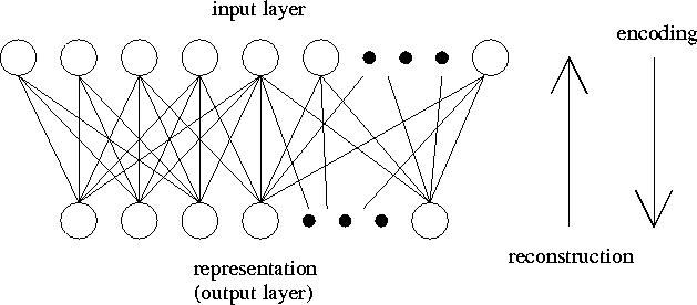
Figure 2.1:
Architecture underlying unsupervised learning models based on
reconstruction error minimisation.
Due to the information loss in mapping ![]() there is no unique
way to choose the reconstruction mapping
there is no unique
way to choose the reconstruction mapping ![]() . This can be
illustrated by considering a linear mapping from 2-dimensional input
. This can be
illustrated by considering a linear mapping from 2-dimensional input
![]() to 1-dimensional output y. The mapping
to 1-dimensional output y. The mapping ![]() is many-to-one, and therefore it does not have a unique inverse. If
we are given the output y, there are many candidate inputs
is many-to-one, and therefore it does not have a unique inverse. If
we are given the output y, there are many candidate inputs
![]() which could have generated the output, thus we have many
possible choices for the reconstruction mapping
which could have generated the output, thus we have many
possible choices for the reconstruction mapping ![]() . There
is no obvious way to know which one of them would minimise the
reconstruction error. If the reconstruction mapping
. There
is no obvious way to know which one of them would minimise the
reconstruction error. If the reconstruction mapping ![]() is
given instead of
is
given instead of ![]() , however, we can simply define the mapping
, however, we can simply define the mapping
![]() to be the one that minimises the reconstruction error.
Among all different possible outputs we choose the one that minimises
the reconstruction error.
to be the one that minimises the reconstruction error.
Among all different possible outputs we choose the one that minimises
the reconstruction error.
In our example this would mean that we first define a linear
reconstruction mapping from y to ![]() and then solve the
and then solve the
![]() that minimises the quadratic reconstruction error. It
turns out that
that minimises the quadratic reconstruction error. It
turns out that ![]() is a unique linear mapping.
is a unique linear mapping.
The example shows how it is often difficult to find the reconstruction
mapping ![]() for a given mapping
for a given mapping ![]() , but
equation 2.1 makes it easy to find the mapping
, but
equation 2.1 makes it easy to find the mapping
![]() from a given reconstruction mapping
from a given reconstruction mapping ![]() . By using
equation 2.1 it is also easy to impose various
constraints on the outputs
. By using
equation 2.1 it is also easy to impose various
constraints on the outputs ![]() , because we can restrict the
search for the minimum in equation 2.1 to the set of
allowed outputs.
, because we can restrict the
search for the minimum in equation 2.1 to the set of
allowed outputs.
A further advantage of using equation 2.1 is that the
derivatives of the reconstruction error with respect to the outputs
are zero because the outputs minimise the reconstruction error. This
greatly simplifies the derivation of the learning rule for the
network. If we denote the parameters of the network by ![]() , then, for a given input
, then, for a given input ![]() , the
reconstruction error is a function of the outputs and the weights:
, the
reconstruction error is a function of the outputs and the weights:
![]() . The goal of the learning is to adapt
the parameters so that the average reconstruction error made by the
network is minimised. We can derive the adaptation rule for the
weights by applying gradient descent. To do this we have to be able
to compute the derivatives of
. The goal of the learning is to adapt
the parameters so that the average reconstruction error made by the
network is minimised. We can derive the adaptation rule for the
weights by applying gradient descent. To do this we have to be able
to compute the derivatives of ![]() with respect to the weights
with respect to the weights
![]() .
.
The last step follows from the fact that in equation 2.1
the outputs are defined to minimise the reconstruction error ![]() and thus
and thus ![]() for all
j. The last step holds even if there were some constraints for the
outputs, which do not depend on the parameters
for all
j. The last step holds even if there were some constraints for the
outputs, which do not depend on the parameters ![]() . Let us denote
. Let us denote
![]() . This vector points to the
direction of the change in the output, when the parameter
. This vector points to the
direction of the change in the output, when the parameter ![]() changes by an infinitesimal amount. If the outputs are constrained,
changes by an infinitesimal amount. If the outputs are constrained,
![]() can only point to a direction where
can only point to a direction where ![]() is
allowed to change. The sum in equation 2.2 can be
interpreted as the directional derivative of
is
allowed to change. The sum in equation 2.2 can be
interpreted as the directional derivative of ![]() in the
direction
in the
direction ![]() . The outputs minimise
. The outputs minimise ![]() and
therefore the derivative is zero in all allowed directions of change
of the outputs.
and
therefore the derivative is zero in all allowed directions of change
of the outputs.
The outputs could, for example, be restricted to be non-negative.
Suppose that the output ![]() would be zero due to this constraint.
If the output had been allowed to be negative, the reconstruction
error could have been further decreased by decreasing
would be zero due to this constraint.
If the output had been allowed to be negative, the reconstruction
error could have been further decreased by decreasing ![]() . This
means that the derivative
. This
means that the derivative ![]() cannot be zero. This time, however, the output
cannot be zero. This time, however, the output ![]() would not change
if the parameters changed only by an infinitesimal amount. The output
would not change
if the parameters changed only by an infinitesimal amount. The output
![]() would still remain exactly zero. Therefore, in this example it
always holds that either
would still remain exactly zero. Therefore, in this example it
always holds that either ![]() or
or
![]() .
.
Problems may arise if equation 2.1 has degenerate
solutions. If we are using the network in feedforward phase, that is,
we are not adapting the parameters, then we can just pick one of the
solutions. We might run into problems if we try to adapt the network,
because the mapping ![]() has discontinuities where the
equation 2.1 has degenerate solutions, and it is not
possible to compute the derivatives of outputs
has discontinuities where the
equation 2.1 has degenerate solutions, and it is not
possible to compute the derivatives of outputs ![]() in
equation 2.2. Luckily in most practical cases the
probability of degenerate solutions is zero.
in
equation 2.2. Luckily in most practical cases the
probability of degenerate solutions is zero.
Equations 2.1 and 2.2 provide us a general framework for developing neural networks based on reconstruction error minimisation. The development starts by defining the reconstruction error, the parametrised reconstruction mapping, and possible constraints for the outputs. Sometimes we are able to solve equation 2.1 in a closed form, but in general we have to solve it numerically.
We shall first consider a simple case where we can find the solution
to equation 2.1 in a closed form. If we require the
reconstruction ![]() to be a linear mapping and there are no
constraints imposed on the outputs, it turns out that, assuming the
quadratic reconstruction error, also the mapping
to be a linear mapping and there are no
constraints imposed on the outputs, it turns out that, assuming the
quadratic reconstruction error, also the mapping ![]() will be
linear. There are many degrees of freedom in the mapping and we can
require the mapping to be orthogonal
will be
linear. There are many degrees of freedom in the mapping and we can
require the mapping to be orthogonal without any loss of generality. The principal
component analysis (PCA) gives this kind of orthogonal mapping
which is optimal with respect to the quadratic reconstruction error
(see e.g. Oja, 1995). The code is maximally dense in
the sense that all the neurons participate in representing any given
input.
(For more
information about PCA see the Master's Thesis of
Jaakko Hollmén).
without any loss of generality. The principal
component analysis (PCA) gives this kind of orthogonal mapping
which is optimal with respect to the quadratic reconstruction error
(see e.g. Oja, 1995). The code is maximally dense in
the sense that all the neurons participate in representing any given
input.
(For more
information about PCA see the Master's Thesis of
Jaakko Hollmén).
If we require the reconstruction to be a linear mapping and
furthermore we require the outputs ![]() to be binary and exactly
one neuron to be active at any one time, then we have made sure that
the code we obtain is maximally local. The resulting coding scheme is
called vector quantisation (VQ) (see e.g. Abut,
1990), because we can simply associate each neuron with the
corresponding reconstruction and then decide the active neuron by
finding the neuron whose reconstruction vector is closest to the input
according to equation 2.1. This can be interpreted as quantifying the input.
to be binary and exactly
one neuron to be active at any one time, then we have made sure that
the code we obtain is maximally local. The resulting coding scheme is
called vector quantisation (VQ) (see e.g. Abut,
1990), because we can simply associate each neuron with the
corresponding reconstruction and then decide the active neuron by
finding the neuron whose reconstruction vector is closest to the input
according to equation 2.1. This can be interpreted as quantifying the input.
When the same basic scheme can produce both maximally dense and local
codes, it is obvious to try to produce also sparse codes. Saund
(1994, 1995) has proposed a few different
reconstruction mappings ![]() , which can be used for sparse
coding. They are chosen so that the resulting coding is sparse
whenever the input is sparse, i.e., is describable with a sparse code.
Unfortunately the inputs have to be binary, which restricts the use of
the algorithm. It might be possible to generalise the approach for
graded inputs, but it does not seem very easy. Olshausen and Field
(1995) have developed an algorithm which uses the
same kind of linear reconstruction scheme as PCA and VQ, but have
added an extra term which promotes sparsity to the reconstruction
error function. Equation 2.1 does not have a simple
closed form solution in either of these algorithms, and the outputs
have to be computed iteratively by gradient descent of the
reconstruction error
, which can be used for sparse
coding. They are chosen so that the resulting coding is sparse
whenever the input is sparse, i.e., is describable with a sparse code.
Unfortunately the inputs have to be binary, which restricts the use of
the algorithm. It might be possible to generalise the approach for
graded inputs, but it does not seem very easy. Olshausen and Field
(1995) have developed an algorithm which uses the
same kind of linear reconstruction scheme as PCA and VQ, but have
added an extra term which promotes sparsity to the reconstruction
error function. Equation 2.1 does not have a simple
closed form solution in either of these algorithms, and the outputs
have to be computed iteratively by gradient descent of the
reconstruction error ![]() . This makes the computational
complexity depend quadratically on the number of the neurons in the
network.
. This makes the computational
complexity depend quadratically on the number of the neurons in the
network.
Although the mappings ![]() and
and ![]() can be related by
using equation 2.1, it is also possible to parametrise
and learn them both separately. Algorithms using this kind of
autoencoder framework have been proposed by several authors, and there
has also been modifications which yield sparse codes
[Dayan and Zemel, 1995, Zemel, 1993, Hinton and Zemel, 1994]. These algorithms can compute the
outputs without any time consuming iterations, but unfortunately
learning seems to be very slow. This is probably due to the fact that
the network has to learn the same things twice as the learning does
not take into account the relation between
can be related by
using equation 2.1, it is also possible to parametrise
and learn them both separately. Algorithms using this kind of
autoencoder framework have been proposed by several authors, and there
has also been modifications which yield sparse codes
[Dayan and Zemel, 1995, Zemel, 1993, Hinton and Zemel, 1994]. These algorithms can compute the
outputs without any time consuming iterations, but unfortunately
learning seems to be very slow. This is probably due to the fact that
the network has to learn the same things twice as the learning does
not take into account the relation between ![]() and
and ![]() in any way.
in any way.