Variational Bayesian Learning

Variational Bayesian (VB) learning provides even stronger tools against overfitting. VB version of PCA [10] approximates the joint posterior of the unknown quantities using a simple multivariate distribution. Each model parameter is described a posteriori using independent Gaussian distributions: $q(a_{ik}) = \mathcal{N}\left(a_{ik};\overline{a}_{ik},\widetilde{a}_{ik}\right)$ and $q(s_{kj}) = \mathcal{N}\left(s_{kj};\overline{s}_{kj},\widetilde{s}_{kj}\right)$, where $\overline{a}_{ik}$ and $\overline{s}_{kj}$ denote the mean of the solution and $\widetilde{a}_{ik}$ and $\widetilde{s}_{kj}$ denote the variance of each parameter. The means $\overline{a}_{ik}$, $\overline{s}_{kj}$ can then be used as point estimates of the parameters while the variances $\widetilde{a}_{ik}$, $\widetilde{s}_{kj}$ define the reliability of the estimates (or credible regions). The direct extension of the method in [10] to missing values can be computationally very demanding. VB-PCA has been used to reconstruct missing values in [11,12] with algorithms that complete the data matrix, which is also very inefficient in case a large part of data is missing. In this article, we implement VB learning using a gradient-based procedure similar to the subspace learning algorithm described in Section 3.

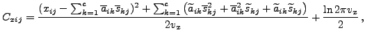
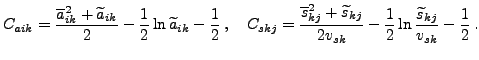
By applying the framework described in [12] to the model in Eqs. (7-8), the cost function becomes:

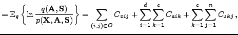$$C_ = \operatorname{E}_q\left\{ \ln\frac{q(\mathbf{A},\mathbf{S})}{p(... ...xij} + \sum_{i=1}^d\sum_{k=1}^c C_{aik} + \sum_{k=1}^c\sum_{j=1}^n C_{skj} \, ,$$ (10)

where individual terms are

$$C_{xij} = \frac{(x_{ij}-\sum_{k=1}^c \overline{a}_{ik}\overline{s... ...detilde{a}_{ik}\widetilde{s}_{kj}\right)}{2 v_x} + \frac{\ln 2 \pi v_x}{2} \, ,$$

$$C_{aik} = \frac{\overline{a}_{ik}^2+\widetilde{a}_{ik}}{2} - \fra... ...- \frac{1}{2}\ln \frac{\widetilde{s}_{kj}}{v_{sk}} - \frac{1}{2} \, . \nonumber$$

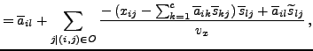
We update $\widetilde{a}$ and $\widetilde{s}$ to minimize the cost by setting the gradient of the cost function to zero:

$$\widetilde{a}_{ik} \leftarrow \left[1+ \sum_{j\mid (i,j)\in O} \f... ...i,j)\in O} \frac{\overline{a}_{ik}^2+\widetilde{a}_{ik}}{v_x} \right]^{-1} \, .$$ (11)

The gradients for learning $\overline{a}$ and $\overline{s}$ are somewhat similar to (4):

$$\frac{\partial C_\text{KL}}{\partial \overline{a}_{il}} = \overline{a}_{il} + \sum_{j\mid (i,j)\in O} \frac{-\left(x_{ij}... ...{kj}\right) \overline{s}_{lj} + \overline{a}_{il} \widetilde{s}_{lj}}{v_x} \, ,$$ (12)

$$\frac{\partial C_\text{KL}}{\partial \overline{s}_{lj}} = \frac{\overline{s}_{lj}}{v_{sk}} + \sum_{i\mid (i,j)\in O} \fra... ...kj}\right) \overline{a}_{il} + \widetilde{a}_{il} \overline{s}_{lj} }{v_x} \, .$$ (13)

We can use the speed-up described in Section 3 by computing the second derivatives. These derivatives happen to coincide with the inverse of the updated variances given in (11): $\partial^2 C_$KL$/ \partial \overline{a}_{il}^2 = \widetilde{a}_{il}^{-1}$ and $\partial^2 C_$KL$/ \partial \overline{s}_{lj}^2 = \widetilde{s}_{lj}^{-1}$. The $v_x$ and $v_s$ parameters are updated to minimize the cost $C_$KL assuming all the other parameters fixed. The complete algorithm works by alternating four update steps: $\{\widetilde{a}\}$, $\{\widetilde{s}\}$, $\{\overline{a},\overline{s}\}$, and $\{v_x, v_{s}\}$.