Regularization

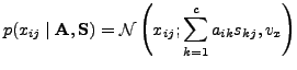
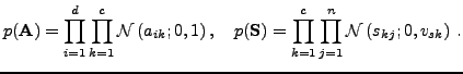
A popular way to regularize ill-posed problems is penalizing the use of large parameter values by adding a proper penalty term into the cost function. This can be obtained using a probabilistic formulation with (independent) Gaussian priors and a Gaussian noise model:

$$p(x_{ij} \mid \mathbf{A},\mathbf{S}) = \mathcal{N}\left(x_{ij};\sum_{k=1}^c a_{ik}s_{kj},v_x\right)$$ (7)

$$p(\mathbf{A}) = \prod_{i=1}^d \prod_{k=1}^c \mathcal{N}\left(a_{i... ...f{S}) = \prod_{k=1}^c \prod_{j=1}^n \mathcal{N}\left(s_{kj};0,v_{sk}\right) \,.$$ (8)

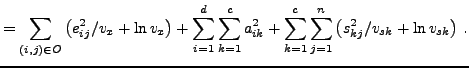
The cost function (ignoring constants) is minus logarithm of the posterior of the unknown parameters:

$$C_ = \sum_{(i,j) \in O} \left( e_{ij}^2/v_x + \ln v_x \right) + \sum... ...k}^2 + \sum_{k=1}^c\sum_{j=1}^n \left(s_{kj}^2/v_{sk} + \ln v_{sk} \right) \, .$$ (9)

The cost function can be minimized using a gradient-based approach as described in Section 3. The corresponding update rules are similar to (5)-(6) except for the extra terms which come from the prior. Note that in case of joint optimization of $C_$BR w.r.t. $a_{ik}$, $s_{kj}$, $v_{sk}$, and $v_x$, the cost function (9) has a trivial minimum with $s_{kj}=0$, $v_{sk}\rightarrow 0$. We try to avoid this minimum by using an orthogonalized solution provided by unregularized PCA for initialization. Note also that setting $v_{sk}$ to small values for some components $k$ is equivalent to removal of irrelevant components from the model. This allows for automatic determination of the proper dimensionality $c$ instead of discrete model comparison (see, e.g., [10]).