Form of the cost function

The form of the part of the cost function that an output of a node affects is shown to be of the form

$${\cal C}_p = M \left< \cdot \right> + V [(\left< \cdot \right>- \... ...rrent}})^2 + \mathrm{Var}\left\{\cdot\right\}] + E\left< \exp \cdot \right> + C$$ (61)

where $\left< \cdot \right>$ denotes the expectation of the quantity in question. If the output is connected directly to another variable, this can be seen from Eq. (10) by substituting

$$M =\left< \exp v \right>(\left< s \right>_{\text{current}}-\left< m \right>)$$

$$V =\frac{1}{2}\left< \exp v \right>$$

$$E =0$$

$$C =\frac{1}{2}\left[\left< \exp v \right>\left(\mathrm{Var}\left\{m... ...^2-\left< s \right>_{\text{current}}^2\right)-\left< v \right>+\ln 2\pi\right].$$

If the output is connected to multiple variables, the sum of the affected costs is of the same form. Now one has to prove that this form remains the same when the signals are fed through the addition and multiplication nodes. ⁵

If the cost function is of the predefined form (61) for the sum $s_1 + s_2$, it has the same form for $s_1$, when $s_2$ is regarded as a constant. This can be shown using Eqs. (20), (21), and (22):

$${\cal C}_p = M\left< s_1+s_2 \right>+ V\left[\left(\left< s_1+s_2 \right> - ... ...2 \right>_{\text{current}}\right)^2 + \mathrm{Var}\left\{s_1+s_2\right\}\right]$$

$$\phantom{=} + E\left< \exp (s_1 + s_2) \right> + C$$ (62)

$$= M\left< s_1 \right> + V\left[\left(\left< s_1 \right>- \left< s_1 \right>_{\text{current}}\right)^2 + \mathrm{Var}\left\{s_1\right\}\right]$$

$$\phantom{=} + (E\left< \exp s_2 \right>)\left< \exp s_1 \right> + \left(C + M\left< s_2 \right> + V \mathrm{Var}\left\{s_2\right\}\right)$$

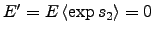It can also be seen from (62) that when $E = 0$ for the sum $s_1 + s_2$, it is zero for the addend $s_1$, that is $E^\prime=E\left< \exp s_2 \right>=0$. This means that the outputs of product and nonlinear nodes can be fed through addition nodes.

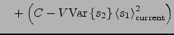
If the cost function is of the predefined form (61) with $E = 0$ for the product $s_1 s_2$, it is similar for the variable $s_1$, when the variable $s_2$ is regarded as a constant. This can be shown using Eqs. (23) and (24):

$${\cal C}_p = M\left< s_1s_2 \right> + V\left[\left(\left< s_1s_2 \right> - \... ...right>_{\text{current}}\right)^2 + \mathrm{Var}\left\{s_1s_2\right\}\right] + C$$ (63)

$$= \left(M\left< s_2 \right> + 2V\mathrm{Var}\left\{s_2\right\}\left< s_1 \right>_{\text{current}}\right)\left< s_1 \right>$$

$$\phantom{=} + \left[V\left(\left< s_2 \right>^2 + \mathrm{Var}\le... ...< s_1 \right>_{\text{current}}\right)^2 + \mathrm{Var}\left\{s_1\right\}\right]$$

$$\phantom{=} + \left(C - V\mathrm{Var}\left\{s_2\right\}\left< s_1 \right>_{\text{current}}^2 \right)$$