The basic idea in variational Bayesian learning
is to minimise the misfit between the exact posterior pdf
 and its parametric approximation
 .
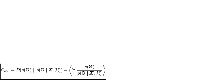
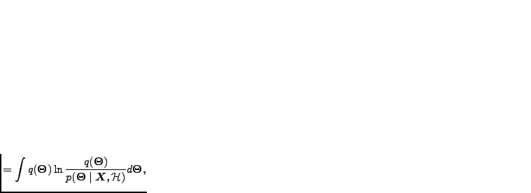
The misfit is measured here with the Kullback-Leibler (KL) divergence
.
The misfit is measured here with the Kullback-Leibler (KL) divergence
 denotes an expectation over the
distribution
. The marginal likelihood
denotes an expectation over the
distribution
. The marginal likelihood
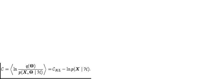
 is hard to evaluate and therefore
the cost function
is hard to evaluate and therefore
the cost function
 that is actually used is
A typical choice of posterior approximations
is Gaussian with
limited covariance matrix, that is, all or most of the off-diagonal
elements are fixed to zero.
Often the posterior approximation is assumed to be a product of independent factors.
The factorial approximation, combined with the
factorisation of the joint probability like in
Equation (3.1), leads to the division of the cost
function in Equation (4.3) into a sum of simple terms, and
thus to a relatively low computational complexity.
Miskin and MacKay (2001) used VB learning for ICA (See Section 3.1.4). They compared two approximations of the posterior: The first was a Gaussian with full covariance matrix, and the second was a Gaussian with a diagonal covariance matrix. They noticed that the factorial approximation is computationally more efficient and still gives a bound on the evidence and does not suffer from overfitting. On the other hand, Ilin and Valpola (2005) showed that the factorial approximation favours a solution that has an orthogonal mixing matrix, which can deteriorate the performance.