Bayesian networks

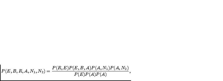
Let us study an example by Pearl (1988). Mr. Holmes receives a phone call from his neighbour about an alarm in his house. As he is debating whether or not to rush home, he remembers that the alarm might have been triggered by an earthquake. If an earthquake had occurred, it might be on the news, so he turns on his radio. The events are shown in Figure 3.1. Marking the events earthquake by $E$, burglary by $B$ and so on, the joint probability can be factored into

$$\begin{multline} P(E,B,R,A,N_1,N_2) = \\ P(E)P(B\mid E)P(R\mid E,B)P(A\mid E,... ... \\ = P(E)P(B)P(R\mid E)P(A\mid E,B)P(N_1\mid A)P(N_2\mid A). \end{multline}$$

The first equation is just basic manipulation of probabilities and the second equation represents conditional independencies. For instance, the probability of an earthquake report on the radio $R$ does not depend on whether there is a burglary $B$ or not, given that we know whether there was an earthquake or not, so $P(R\mid E,B)=P(R\mid E)$.

Figure 3.1: Top left: Bayesian network for the alarm example. Top right: A Markov network formed by connecting all parents that share a common child and removing edge directions. Bottom: The corresponding join tree whose nodes correspond to cliques of the Markov network.

The graphical representation of the conditional probabilities depicted in the top left subfigure of Figure 3.1 is intuitive: arrows point from causes to effects. Note that the graph has to be acyclic, no occurrence can be its own cause. Loops, or cycles when disregarding directions of the edges, are allowed. Assuming that the variables are discrete, the conditional probabilities are described using a conditional probability table that lists probabilities for all combinations of values for the relevant variables. For instance, $P(N_1\mid A)$ is described in Table 3.1. Recalling the notation from Section 2.3, the numbers in the conditional probability table are parameters $\boldsymbol{\theta}$ while unobserved variables in the nodes are $\boldsymbol{S}$.

Table 3.1: The conditional probability table describing $P(N_1\mid A)$.

	$N_1$=true	$N_1$=false
$A$=true	$0.7$	$0.3$
$A$=false	$0.001$	$0.999$

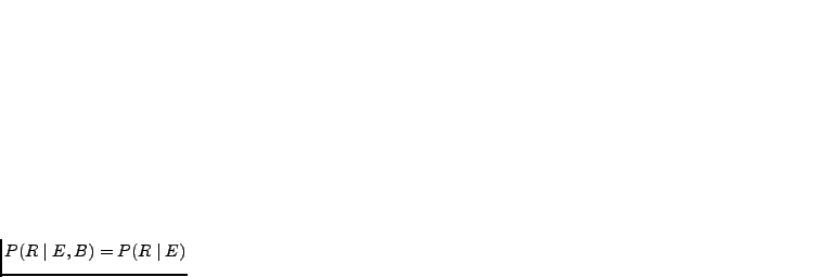
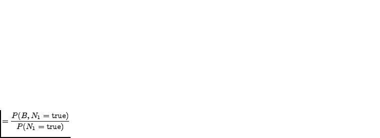
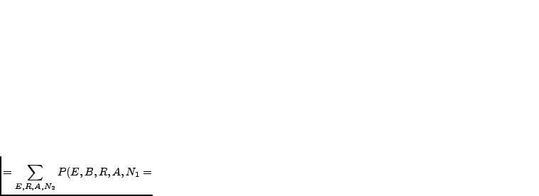
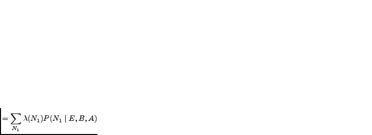
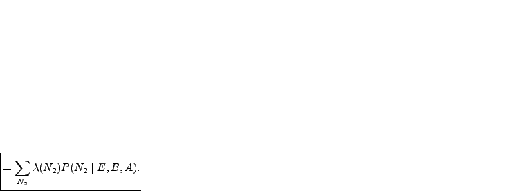
Inference in Bayesian networks solves questions such as ``what is the probability of burglary given that neighbour 1 calls about the alarm?'' Approximate inference methods such as sampling (see Section 2.5.4) can be used, but in relatively simple cases, also exact inference can be done. For that purpose, we will form the join tree of the Bayesian network. First, we connect parents of a node to each other, and remove all directions of the edges, (see top right subfigure of Figure 3.1). This is called a Markov network. Next, we find all cliques (fully connected subgraphs) of the Markov network. Then we create a join tree^3.1 where nodes represent the cliques in the Markov network and edges are set between nodes who share some variables (see bottom subfigure of Figure 3.1).

We can rewrite the joint distribution in Equation 3.1 as

$$P(E,B,R,A,N_1,N_2) = \frac{P(R,E)P(E,B,A)P(A,N_1)P(A,N_2)}{P(E)P(A)P(A)},$$ (3.1)

where the numerator is a product of distributions of nodes in the join tree and the denominator is the product of the distributions of the edges of the join tree. Then the inference question ``what is the probability of burglary given that neighbour 1 calls about the alarm?'' is solved by substituting $N_1=true$ and marginalising the uninteresting variables away:

$$P(B\mid N_1= ) = \frac{P(B,N_1=\text{true})}{P(N_1=\text{true})}$$

$$\propto P(B,N_1= )$$

$$= \sum_{E,R,A,N_2} P(E,B,R,A,N_1= ,N_2)$$

$$= \sum_{E,R,A,N_2} \frac{P(R,E)P(E,B,A)P(A,N_1=\text{true})P(A,N_2)}{P(E)P(A)P(A)},$$ (3.2)

where $\propto$ means ``proportional to''. The constant $P(N_1=$true$)$ can be ignored if the resulting distribution is normalised in the end. Summing over all the latent variables is often prohibitively computationally expensive, so better means have been found.

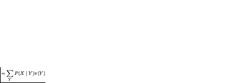
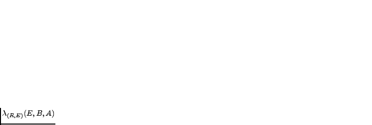
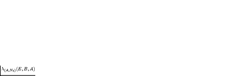
For efficient marginalisation in join trees, there is an algorithm called belief propagation (Pearl, 1988) based on message passing. First, any one of the nodes in the join tree is selected as a root. Messages $\pi$ are sent away from the root and messages $\lambda$ towards the root. The marginal posterior probability of a node $X$ in the join tree given observations ${\bf e}$ is decomposed into two parts:

$$P(X\mid {\bf e}) \propto P(X\mid {\bf e}_ ) P({\bf e}_ \mid X)$$

$$= \pi(X)\lambda(X),$$ (3.3)

where ${\bf e}_$anc(X) and ${\bf e}_$desc(X) are the observations in the ancestor and descendant nodes of $X$ in the join tree accordingly. The messages can be computed recursively by

$$\pi(X) = \sum_{Y} P(X\mid Y) \pi(Y)$$ (3.4)

$$\lambda(Y) = \prod_j \lambda_j(Y)$$ (3.5)

$$\lambda_X(Y) = \sum_X \lambda(X)P(X\mid Y)$$ (3.6)

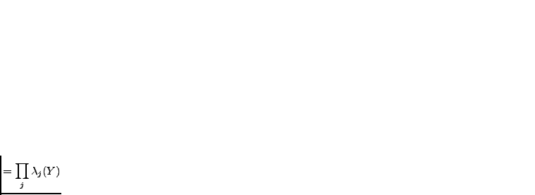
where $Y$ is the parent of $X$ in the join tree and $j$ are its children, including $X$. The message $\pi$ for the root node is set to the prior probability of the node, and the messages $\lambda$ are set to uniform distribution for the unobserved leaf nodes. The belief propagation algorithm extended for logical hidden Markov models in Publication VII.

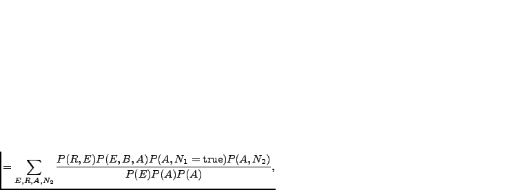
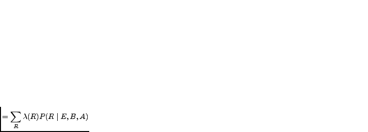
Returning to the example in Equation 3.2 and selecting node $(E,B,A)$ as the root of the join tree, the necessary messages are

$$\pi(E,B,A) = P(E,B,A)$$ (3.7)

$$\lambda_{(R,E)}(E,B,A) = \sum_R \lambda(R)P(R\mid E,B,A)$$ (3.8)

$$\lambda_{(A,N_1)}(E,B,A) = \sum_{N_1} \lambda(N_1)P(N_1\mid E,B,A)$$ (3.9)

$$\lambda_{(A,N_2)}(E,B,A) = \sum_{N_2} \lambda(N_2)P(N_2\mid E,B,A).$$ (3.10)

Since $\lambda(R)$ and $\lambda(N_2)$ are uniform (unobserved leaf nodes), it is easy to see that $\lambda_{(R,E)}(E,B,A)$ and $\lambda_{(A,N_2)}(E,B,A)$ are also uniform and can thus be ignored. We get

$$P(B\mid N_1= ) = \sum_{E,A} \pi(E,B,A)\lambda(E,B,A)$$

$$= \sum_{E,A} P(E,B,A)\lambda_{(A,N_1)}(E,B,A)$$

$$= \sum_{E,A} P(E,B,A) P(N_1= \mid E,B,A)$$

$$= \sum_{E,A} P(E)P(B)P(A\mid E,B) P(N_1= \mid A).$$ (3.11)

For the inference to be exact, the join tree must not have loops (like the name implies). Loopy belief propagation by Murphy et al. (1999) uses belief propagation algorithm regardless of loops. Experiments show that in many cases it still works fine. The messages are initialised uniformly and iteratively updated until the process hopefully converges. It is also possible to find an exact solution by getting rid of loops at the cost of increased computational complexity. This happens by adding edges to the Markov network.

Bayesian networks can manage continuous valued variables, when three simplifying assumptions are made (Pearl, 1988). All interactions between variables are linear, the sources of uncertainty are normally distributed, and the causal network is singly connected (no two nodes share both common descendants and common ancestors). Instead of tables, the conditional probabilities are described with linear mappings. Posterior probability is Gaussian.

Bayesian networks are static, that is, each data sample is independent from others. The extension to dynamic (or temporal) Bayesian networks (see Ghahramani, 1998) is straightforward. Assume that the data samples $\mathbf{x}$, e.g.  $\mathbf{x}=(E,B,R,A,N_1,N_2)$, are indexed by time $t$. Each variable can have as parents variables of sample $\mathbf{x}(t-1)$ in addition to the variables of the sample itself $\mathbf{x}(t)$. Hidden Markov models (see Section 3.1.5) are an important special case of dynamic Bayesian networks.

Linearity assumption can be relaxed when some approximations are made. Section 4.4 and Publication I present such a framework based on variational Bayesian learning. There are also other approaches. Hofmann and Tresp (1996) study Bayesian networks with nonlinear conditional density estimators. Inference is based on Gibbs sampling and learning is based on cross-validated maximum a posteriori estimation.