Independent component analysis

The mixing model of independent component analysis (ICA) is similar to that of the FA (see Figure 3.2), but in the basic case with equal number of factors (or components) as observations and without the noise term. The data is thought to have been generated from independent components $\mathbf{s}(t)$ through a square mixing matrix $\mathbf{A}$ by

$$\mathbf{x}(t) = \mathbf{A}\mathbf{s}(t) .$$ (3.18)

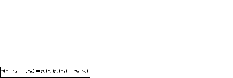
The components $\mathbf{s}(t)$ are independent, that is,

$$p(s_1,s_2,\dots,s_n) = p_1(s_1)p_2(s_2)\dots p_n(s_n),$$ (3.19)

and the assumption of Gaussianity of the components is relaxed. Assuming that at most one of the independent components is Gaussian, the model is identifiable (Comon, 1994).

In the basic case, the number of components is the same as the number of observation and the components can be reconstructed from data given the mixing matrix $\mathbf{A}$ by $\mathbf{s}(t)=\mathbf{A}^{-1}\mathbf{x}(t)$. The independence of the reconstructed $\mathbf{s}(t)$ can then be measured for instance by the non-Gaussianity of the components or by mutual information (Hyvärinen et al., 2001). ICA can thus be done by iteratively maximising such a measure. ICA has many fields of applications, such as brain imaging (Vigário et al., 1998), telecommunications (Raju et al., 2006; Ristaniemi, 2000), speech separation, and so on (Hyvärinen et al., 2001).

ICA can be approached from different starting points. It can be viewed as a Bayesian network when the one dimensional distributions for the components are modelled with for example mixtures-of-Gaussians (Miskin and MacKay, 2001; Attias, 2001,1999; Choudrey et al., 2000). This is also known as independent factor analysis. Extensions to the basic ICA involve additive noise, convolutive or nonlinear mixing, and the number of components might differ from the number of observations (Hyvärinen et al., 2001).

Publication III studies the reconstruction of corrupted values in data by independent factor analysis.