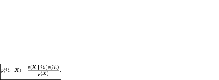
VB learning offers another important benefit. Comparison of different models is straightforward. The Bayes rule can be applied again to get the probability of a model given the data
 is the prior probability of the model
 and
and
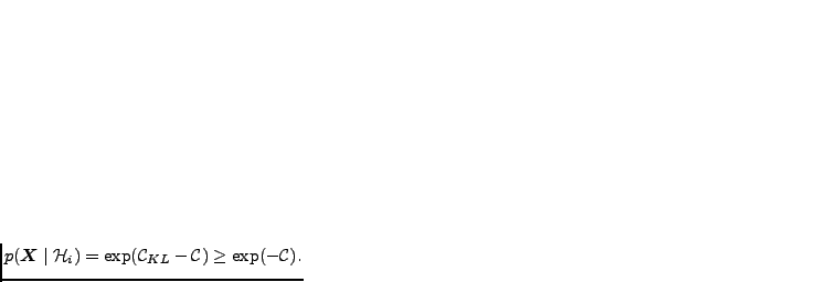
 is a constant that can be ignored. A lower bound on the
evidence term
is a constant that can be ignored. A lower bound on the
evidence term
 is obtained from Equation (4.3) and it is
Multiple models can be used as a mixture-of-experts model
(Haykin, 1999). The experts can be weighted with their probabilities
 given in equation
(4.4). Lappalainen and Miskin (2000) show that the
optimal weights in the sense of variational Bayesian approximation are
in fact
given in equation
(4.4). Lappalainen and Miskin (2000) show that the
optimal weights in the sense of variational Bayesian approximation are
in fact
 . If the models have equal prior
probabilities
, the weights simplify further to
. If the models have equal prior
probabilities
, the weights simplify further to
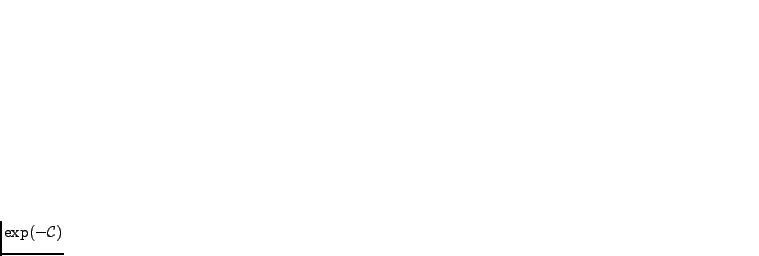 . In practice, the costs
 tend to differ in the order of
hundreds or thousands, which makes the model with the lowest cost
dominant. Therefore it is reasonable to concentrate on model
selection rather than weighting.
tend to differ in the order of
hundreds or thousands, which makes the model with the lowest cost
dominant. Therefore it is reasonable to concentrate on model
selection rather than weighting.