Nonlinear Artificial Data

The cost function which is based on ensemble learning and which the algorithm tries to minimise can be interpreted as the description length of the data [3]. The following experiments show that the cost function can be used for optimising the structure of the MLP network in addition to learning the unknown variables of the model.

This data set of 1000 vectors was generated by a randomly initialised MLP network with five inputs, 20 hidden neurons and ten outputs. The inputs were all normally distributed. Gaussian noise with standard deviation 0.1 was added to the data. The nonlinearity for the hidden neurons was chosen to be the inverse hyperbolic sine, while the MLP network which was estimated by the algorithm had hyperbolic tangent as its nonlinearity.

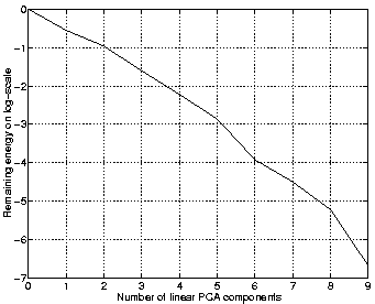
**Figure 2:** Remaining energy in the data as a function of extracted linear PCA components.
$\begin{figure}\begin{center} \epsfig{file=linpcaerr.eps,width=7.5cm} \end{center} \end{figure}$

Figure 2 shows how much of the energy remains in the data when a number of linear PCA components are extracted. This measure is often used to infer the linear dimension of the data. As the figure shows, there is no obvious turn in the curve and it is difficult to tell what the linear dimension is. At least it is not five which is the underlying nonlinear dimension of the data.

**Figure 3:** Several different initialisations of the MLP network were tested and the smallest attained value of the cost function is shown for each number of hidden neurons.
$\begin{figure}\begin{center} \epsfig{file=nlpcahid.eps,width=7cm} \end{center} \end{figure}$

**Figure 4:** Several different initialisations of the MLP network were tested and the smallest attained value of the cost function is shown for each number of sources.
$\begin{figure}\begin{center} \epsfig{file=nlpcasrc.eps,width=7cm} \end{center} \end{figure}$

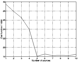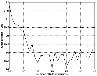
With the nonlinear IFA by MLP networks, not only the number of sources but also the number of hidden neurons needs to be estimated. With the cost function based on ensemble learning this is not a problem as is seen in Figs. 3 and 4. The cost function exhibits a broad minimum as a function of the number of hidden neurons and saturates after five sources when plotted as a function of sources.

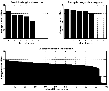
The value of the cost function can be interpreted as the description length of the whole data. It is also possible to have a closer look at the terms of the cost function and interpret them as the description lengths of individual parameters [3]. The amount of bits which the network has used for describing a parameter can then be used to judge whether the parameter can be pruned away.

**Figure 5:** Average number of bits used by the network to describe various variables.
$\begin{figure}\epsfig{file=bignet.eps,width=8.3cm} \end{figure}$

Figure 5 shows average description lengths for different variables when the data was the same as in previous simulation and an MLP network with seven inputs and 100 hidden neurons was used for estimating the sources. Clearly only five out of seven sources were used by the network. However, only a few hidden neurons were effectively pruned which shows that there is not much pressure for the network to prune away extra hidden neurons. The overall value of the cost function was higher than for models with equal number of sources but fewer hidden neurons.