Helix

  

Figure 1: The noisy data points are shown on the left and the outputs of the MLP network (points) together with the underlying helical subspace (solid line) are shown on the right.

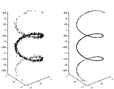
We start with a toy problem which is easy to visualise. A set of 1000 data points, shown on the left of Fig. 1, was generated from a normally distributed source s into a helical subspace. The mapping onto x-, y- and z-axes were $x = \sin(\pi s)$, $y = \cos(\pi s)$ and z=s. Gaussian noise with standard deviation 0.05 was added to all three data components.

Several different initialisations of the MLP networks with different number of hidden neurons were tested and the network which produced the lowest value of the cost function was chosen. The best network had 16 hidden neurons and it had estimated the noise level of different data components to be 0.052, 0.055 and 0.050. The outputs of the network for each estimated value of the source signal¹ together with the original helical subspace are shown on the right of Fig.1. It is evident that the network has learned to represent the underlying one-dimensional subspace and has been able to separate the signal from noise.