Next: Simulation Results
Up: Experiments
Previous: Simulation
The NDFA package version 0.9.5, the scripts for running the experiments, and the used training data are publicly available![[*]](http://www.cis.hut.fi/share/latex2html//footnote.gif) .
During the training phase for indirect methods, training data with
2500 samples was used. In [18], different
reinforcement learning algorithms require from 9000 up to 2500000 samples
to learn to control the cart. Most of the training data consisted of a sequence generated with
semi-random control where the only goal was to ensure that the cart
does not crash into the boundaries. Training data also contained some
examples of hand-generated sections to better model the whole range of
the observation and the dynamic mapping. The model was trained for
500000 iterations, which translates to three days of computation
time. Six-dimensional state space
.
During the training phase for indirect methods, training data with
2500 samples was used. In [18], different
reinforcement learning algorithms require from 9000 up to 2500000 samples
to learn to control the cart. Most of the training data consisted of a sequence generated with
semi-random control where the only goal was to ensure that the cart
does not crash into the boundaries. Training data also contained some
examples of hand-generated sections to better model the whole range of
the observation and the dynamic mapping. The model was trained for
500000 iterations, which translates to three days of computation
time. Six-dimensional state space
 was used because
it resulted in a model with the lowest cost function (Eq. 5).
For the direct control method, training data consisted of 30 examples
of successful swing-ups with 100 samples each. They were generated
using the NMPC method with a horizon length of 40 time steps.
Four-dimensional state space proved to be the best here, and the model was
trained for 100000 iterations.
For all the models, the first 1000 iterations of the training were run
with the embedded versions of the data to avoid bad local
optima. Time-shifted versions of the observed data
was used because
it resulted in a model with the lowest cost function (Eq. 5).
For the direct control method, training data consisted of 30 examples
of successful swing-ups with 100 samples each. They were generated
using the NMPC method with a horizon length of 40 time steps.
Four-dimensional state space proved to be the best here, and the model was
trained for 100000 iterations.
For all the models, the first 1000 iterations of the training were run
with the embedded versions of the data to avoid bad local
optima. Time-shifted versions of the observed data
 ,
with
,
with
 , were used in addition to the original data.
The state
was estimated using the iterated extended
Kalman smoother. A history of five observations and control signals
seemed to suffice to give a reliable estimate. The reference signal
, were used in addition to the original data.
The state
was estimated using the iterated extended
Kalman smoother. A history of five observations and control signals
seemed to suffice to give a reliable estimate. The reference signal
 was
was  and
and  at the end of the horizon
and for five observations beyond that.
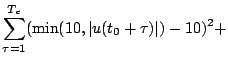
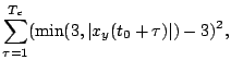
To take care of the constraints in the system with NMPC, a slightly
modified version of the cost function (9) was
used. Out-of-bounds values of the location of the cart and the force
incurred a quadratic penalty, and the full cost function is of the
form
at the end of the horizon
and for five observations beyond that.
To take care of the constraints in the system with NMPC, a slightly
modified version of the cost function (9) was
used. Out-of-bounds values of the location of the cart and the force
incurred a quadratic penalty, and the full cost function is of the
form
where  refers to the location component
  of the observation
vector
of the observation
vector
 .
.
Next: Simulation Results
Up: Experiments
Previous: Simulation
Tapani Raiko
2005-05-23