


Next: Experiments
Up: Natural Conjugate Gradient in
Previous: Natural conjugate gradient
VB for nonlinear state-space models
As a specific example, we consider the nonlinear state-space model
(NSSM) introduced in [5]. The model is specified by
the generative model
where  is time,
 are the observations, and
 are the
hidden states. The observation mapping
are the
hidden states. The observation mapping
 and the dynamical
mapping
and the dynamical
mapping
 are nonlinear and they are modeled with multilayer
perceptron (MLP) networks. Observation noise
are nonlinear and they are modeled with multilayer
perceptron (MLP) networks. Observation noise
 and process noise
 are assumed Gaussian. The latent states
are
commonly denoted by
are assumed Gaussian. The latent states
are
commonly denoted by
 . The model parameters include both
the weights of the MLP networks and a number of hyperparameters. The
posterior approximation of these parameters is a Gaussian with a
diagonal covariance. The posterior approximation of the states
. The model parameters include both
the weights of the MLP networks and a number of hyperparameters. The
posterior approximation of these parameters is a Gaussian with a
diagonal covariance. The posterior approximation of the states
 is a Gaussian Markov random field a correlation between the
corresponding components of subsequent state vectors
is a Gaussian Markov random field a correlation between the
corresponding components of subsequent state vectors
 and
and  .
This is a realistic minimum assumption
for modeling the dependence of the state vectors
and
.
This is a realistic minimum assumption
for modeling the dependence of the state vectors
and
 [5].
[5].
Because of the nonlinearities the model is not in the conjugate
exponential family, and the standard VB learning methods are only
applicable to hyperparameters and not the latent states or
weights of the MLPs. The bound (1) can nevertheless be
evaluated by linearizing the MLP networks
and
using the
technique of [7]. This allows evaluating
the gradient with respect to
 ,
,
 , and
, and
 and using a gradient based optimizer to adapt the
parameters. The natural gradient for the mean elements
is given by
and using a gradient based optimizer to adapt the
parameters. The natural gradient for the mean elements
is given by
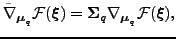 |
(17) |
where
 is the mean of the variational approximation
 and
and
 is the
corresponding covariance. The covariance of the model parameters is
diagonal while the inverse covariance of the latent states
is
block-diagonal with tridiagonal blocks. This implies that all
computations with these can be done in linear time with respect to the
number of the parameters.
The covariances were updated separately using
a fixed-point update rule similar to (2)
as described in [5].
is the
corresponding covariance. The covariance of the model parameters is
diagonal while the inverse covariance of the latent states
is
block-diagonal with tridiagonal blocks. This implies that all
computations with these can be done in linear time with respect to the
number of the parameters.
The covariances were updated separately using
a fixed-point update rule similar to (2)
as described in [5].
Next: Experiments
Up: Natural Conjugate Gradient in
Previous: Natural conjugate gradient
Tapani Raiko
2007-09-11