Experiments

As an example, the method for learning nonlinear state-space models presented in Sec. 5 was applied to real world speech data. Experiments were made with different data sizes to study the performance differences between the algorithms. The data consisted of 21 dimensional mel frequency log power speech spectra of continuous human speech.

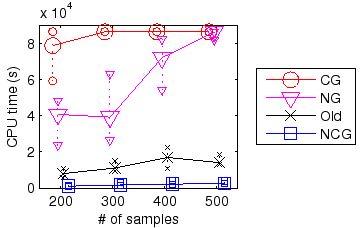
To study the performance differences between the natural conjugate gradient (NCG) method, standard natural gradient (NG) method, standard conjugate gradient (CG) method and the heuristic algorithm from [5], the algorithms were applied to different sized parts of the speech data set. Unfortunately a reasonable comparison with a VB EM algorithm was impossible because the E-step failed due to instability of the used Kalman filtering algorithm.

The size of the data subsets varied between 200 and 500 samples. A five dimensional state-space was used. The MLP networks for the observation and dynamical mapping had 20 hidden nodes. Four different initializations and two different segments of data of each size were used, resulting in eight repetitions for each algorithm and data size. The results for different data segments of the same size were pooled together as the convergence times were in general very similar. An iteration was assumed to have converged when $\vert\mathcal{B}^t-\mathcal{B}^{t-1}\vert< \varepsilon = (10^{-5} N / 500)$ for 5 consecutive iterations, where $\mathcal{B}^t$ is the bound on marginal log-likelihood at iteration $t$ and $N$ is the size of the data set. Alternatively, the iteration was stopped after 24 hours even if it had not converged. Practically all the simulations converged to different local optima, but there were no statistically significant differences in the bound values corresponding to these optima (Wilcoxon rank-sum test, 5 % significance level). There were still some differences, and especially the NG algorithm with smaller data sizes often appeared to converge very early to an extremely poor solution. These were filtered by removing results where the attained bound value that was more than two NCG standard deviations worse than NCG average for the particular data set. The results of one run where the heuristic algorithm diverged were also discarded from the analysis.

The results can be seen in Figure 2. The plain CG and NG methods were clearly slower than others and the maximum runtime was reached by most CG and some NG runs. NCG was clearly the fastest algorithm with the heuristic method between these extremes.

Figure 2: Convergence speed of the natural conjugate gradient (NCG), the natural gradient (NG) and the conjugate gradient (CG) methods as well as the heuristic algorithm (Old) with different data sizes. The lines show median times with 25 % and 75 % quantiles shown by the smaller marks. The times were limited to at most 24 hours, which was reached by a number of simulations.

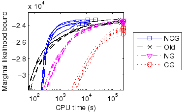
As a more realistic example, a larger data set of 1000 samples was used to train a seven dimensional state-space model. In this experiment both MLP networks of the NSSM had 30 hidden nodes. The convergence criterion was $\varepsilon = 10^{-6}$ and the maximum runtime was 72 hours. The performances of the NCG, NG, CG methods and the heuristic algorithm were compared. The results can be seen in Figure 3. The results show the convergence for five different initializations with markers at the end showing when the convergence was reached.

NCG clearly outperformed the other algorithms in this experiment as well. In particular, both NG and CG hit the maximum runtime in every run, and especially CG was nowhere near convergence at this time. NCG also outperformed the heuristic algorithm [5] by a factor of more than 10.

Figure: Comparison of the performance of the natural conjugate gradient (NCG), the natural gradient (NG), the conjugate gradient (CG) methods and the heuristic algorithm with the full data set. Lower bound on marginal log-likelihood $\mathcal{B}$ is plotted against computation time using a logarithmic time scale. The tick marks show when simulations either converged or were terminated after 72 hours.