Variational Bayesian learning [1,5]
is based on approximating the posterior
distribution
![]() with a tractable approximation
with a tractable approximation
![]() , where
, where
![]() is the data,
is the data,
![]() are the unknown variables
(including both the parameters of the model and the latent variables),
and
are the unknown variables
(including both the parameters of the model and the latent variables),
and
![]() are the variational parameters of the approximation (such as the
mean and the variance of a Gaussian variable). The
approximation is fitted by maximizing a lower bound on marginal log-likelihood
are the variational parameters of the approximation (such as the
mean and the variance of a Gaussian variable). The
approximation is fitted by maximizing a lower bound on marginal log-likelihood
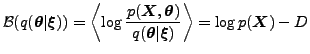 KL KL |
(1) |
Finding the optimal approximation can be seen as an optimization
problem, where the lower bound
![]() is maximized with
respect to the variational parameters
is maximized with
respect to the variational parameters
![]() . This is often solved
using a VB EM algorithm by updating sets of parameters
alternatively while keeping the others fixed. Both VB-E and VB-M steps
can implicitly optimally utilize the Riemannian structure of
. This is often solved
using a VB EM algorithm by updating sets of parameters
alternatively while keeping the others fixed. Both VB-E and VB-M steps
can implicitly optimally utilize the Riemannian structure of
![]() for conjugate exponential family models [10].
Nevertheless, the EM based methods are prone to slow convergence, especially
under low noise, even though more elaborate optimization schemes can
speed up their convergence somewhat.
for conjugate exponential family models [10].
Nevertheless, the EM based methods are prone to slow convergence, especially
under low noise, even though more elaborate optimization schemes can
speed up their convergence somewhat.
The formulation of VB as an optimization problem allows applying
generic optimization algorithms to maximize
![]() , but this
is rarely done in practice because the problems are quite high
dimensional. Additionally other parameters may influence the effect
of other parameters and the lack of this specific knowledge of the
geometry of the problem can seriously hinder generic optimization
tools.
, but this
is rarely done in practice because the problems are quite high
dimensional. Additionally other parameters may influence the effect
of other parameters and the lack of this specific knowledge of the
geometry of the problem can seriously hinder generic optimization
tools.
Assuming the approximation
![]() is Gaussian, it is
often enough to use generic optimization tools to update the mean of
the distribution. This is because the negative entropy of a Gaussian
is Gaussian, it is
often enough to use generic optimization tools to update the mean of
the distribution. This is because the negative entropy of a Gaussian
![]() with mean
with mean
![]() and covariance
and covariance
![]() is
is
![]() and thus straightforward differentiation of
Eq. (1) yields a fixed point update rule for the
covariance
and thus straightforward differentiation of
Eq. (1) yields a fixed point update rule for the
covariance