

Next: Learning Procedure
Up: Hierarchical Nonlinear Factor Analysis
Previous: Results
Experiments with Image Data
HNFA+VM, presented in Chapter ![[*]](cross_ref_motif.gif) , was tested
with a number of natural gray-scale images as a data set.
Gaussian noise with standard deviation 0.1 was added to the images
to avoid artefacts caused by the discrete gray levels from 0 to
255. The intensities were scaled to variance one.
, was tested
with a number of natural gray-scale images as a data set.
Gaussian noise with standard deviation 0.1 was added to the images
to avoid artefacts caused by the discrete gray levels from 0 to
255. The intensities were scaled to variance one.
10 times 10 image patches were taken randomly from the images to be
used as data vectors. There was a total of 10000 data vectors.
The data matrix
X is thus 100 by 10000. The mean of each
patch was subtracted from the patch and the data was whitened to a
degree
 and rotated back to the original space:
 |
(8.1) |
where
V contains the orthonormal eigenvectors of the
covariance matrix of the data and
D is the diagonal matrix of
its eigenvalues. Regular whitening corresponds to  and
whitening to a degree 0 would leave the data unchanged. The partly
whitened version of the data was rotated back to the original space by
multiplying with
VT from the left so that the dimensions of
the data would still correspond to the pixels. Whitening is used,
because the dominating feature of the images is the positive
correlation between nearby pixels and the model could otherwise spend
a layer just to model that. Regular whitening is typically used as a
preprocessing for ICA.
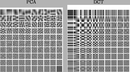
Figure ![[*]](cross_ref_motif.gif) shows the matrix
V or the
principal components of the data. There are only 99 components, since
the removal of the mean in each image removes also one of the
intrinsic dimensions. There is a great resemblance to the discrete
cosine transform (DCT), which is widely used in image compression
[21]. Compression and ensemble learning have much in
common as was seen in Subsection
shows the matrix
V or the
principal components of the data. There are only 99 components, since
the removal of the mean in each image removes also one of the
intrinsic dimensions. There is a great resemblance to the discrete
cosine transform (DCT), which is widely used in image compression
[21]. Compression and ensemble learning have much in
common as was seen in Subsection ![[*]](cross_ref_motif.gif) . Taking into account
that there are efficient algorithms for calculating the DCT, it is
clearly a good choice for compression. None of the patches are
localised in either PCA or DCT.
. Taking into account
that there are efficient algorithms for calculating the DCT, it is
clearly a good choice for compression. None of the patches are
localised in either PCA or DCT.
Figure:
Left: The mixing matrix resulting from applying Principal
Component Analysis (PCA) to the same data set. Right: the basis
of the Discrete Cosine Transform (DCT) that is used in image
compression.
 |


Next: Learning Procedure
Up: Hierarchical Nonlinear Factor Analysis
Previous: Results
Tapani Raiko
2001-12-10
![[*]](cross_ref_motif.gif) , was tested
with a number of natural gray-scale images as a data set.
Gaussian noise with standard deviation 0.1 was added to the images
to avoid artefacts caused by the discrete gray levels from 0 to
255. The intensities were scaled to variance one.
, was tested
with a number of natural gray-scale images as a data set.
Gaussian noise with standard deviation 0.1 was added to the images
to avoid artefacts caused by the discrete gray levels from 0 to
255. The intensities were scaled to variance one.
