

Next: Experiments with Image Data
Up: Bars Problem
Previous: Learning Procedure
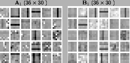
The initial weights of the first layer can be seen in
Figure ![[*]](cross_ref_motif.gif) . Some regular bars are visible, but
there are multiple bars in the same patch. Variance bars are even less
clear. There are a few sources that diminish variance, which means
that they are active when neither of the orientations were in the
generation process.
. Some regular bars are visible, but
there are multiple bars in the same patch. Variance bars are even less
clear. There are a few sources that diminish variance, which means
that they are active when neither of the orientations were in the
generation process.
Figure 7.2:
Posterior means of the weight matrices after 20 sweeps. The second
layer has just been initialised. The matrices are organised in
patches and dark shades represent positive values.
 |
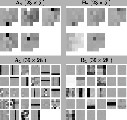
Figure ![[*]](cross_ref_motif.gif) shows the weights after adding
another layer. Regular bars are quite well formed in
A1. Two
sources represent the same rightmost vertical bar, though. The upper
horizontal variance bar and the right vertical variance bar are
somewhat mixed up in
B1. The leftmost source on the second
row clearly diminishes variance. The weights
A2 and
B2 of the upper layer seem to be quite useless at this stage.
shows the weights after adding
another layer. Regular bars are quite well formed in
A1. Two
sources represent the same rightmost vertical bar, though. The upper
horizontal variance bar and the right vertical variance bar are
somewhat mixed up in
B1. The leftmost source on the second
row clearly diminishes variance. The weights
A2 and
B2 of the upper layer seem to be quite useless at this stage.
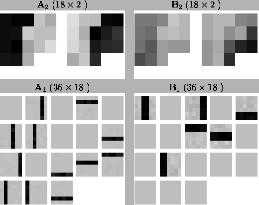
Figure:
Posterior means of the weight matrices after 100 sweeps. The third
layer has just been initialised. The five patches in
A2 and
B2 correspond to the five sources on the third
layer. The pixels of
A2 and
B2 correspond to
the 18 sources on the second layer and thus to the patches of
A1 and
B1.
 |
Figure ![[*]](cross_ref_motif.gif) demonstrates that the algorithm
finds a generative model, that is quite similar to the generation
process. The two sources on the third layer correspond to the
horizontal and vertical orientations and the 18 sources on the second
layer correspond to the bars. Regular bars, present in
A1, are reconstructed accurately but the variance bars in
B1 exhibit some noise. The distinction between horizontal
and vertical orientations is clearly visible in
A2.
demonstrates that the algorithm
finds a generative model, that is quite similar to the generation
process. The two sources on the third layer correspond to the
horizontal and vertical orientations and the 18 sources on the second
layer correspond to the bars. Regular bars, present in
A1, are reconstructed accurately but the variance bars in
B1 exhibit some noise. The distinction between horizontal
and vertical orientations is clearly visible in
A2.
Figure:
Final results: Posterior means of the weight matrices after 1200
sweeps. The sources of the second layer are ordered for
visualisation purposes according to the weights
A2 and
B2 using self-organising map.
 |
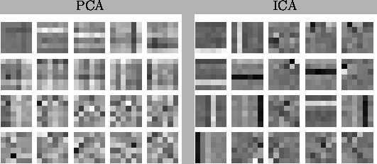
Figure ![[*]](cross_ref_motif.gif) shows the mixing matrices from principal
component analysis (PCA) and independent component analysis (ICA) with
the same data. It should be noted that in PCA and in ICA, there is a
symmetry between dark and light shades and it is irrelevant, which one
is shown. These models are not rich enough to find variance bars. The
regular bars, however, are found to a degree. In PCA, the bars are
mixed up especially with other bars of the same orientation. There
should be 12 bar patches, but the last ones are crippled with
noise. ICA does not mix the bars with each other so much. There are no
mixtures of horizontal and vertical bars. Only ten patches show bars
which means that some must be missing. Results with vector
quantisation (VQ) are practically the ones used in the initialisation
shown in Figure
shows the mixing matrices from principal
component analysis (PCA) and independent component analysis (ICA) with
the same data. It should be noted that in PCA and in ICA, there is a
symmetry between dark and light shades and it is irrelevant, which one
is shown. These models are not rich enough to find variance bars. The
regular bars, however, are found to a degree. In PCA, the bars are
mixed up especially with other bars of the same orientation. There
should be 12 bar patches, but the last ones are crippled with
noise. ICA does not mix the bars with each other so much. There are no
mixtures of horizontal and vertical bars. Only ten patches show bars
which means that some must be missing. Results with vector
quantisation (VQ) are practically the ones used in the initialisation
shown in Figure ![[*]](cross_ref_motif.gif) . Some bars are found well,
but some are missing and some patches are mixtures of horizontal and
vertical bars.
. Some bars are found well,
but some are missing and some patches are mixtures of horizontal and
vertical bars.
Figure:
The mixing matrices found by PCA and ICA algorithms.
 |


Next: Experiments with Image Data
Up: Bars Problem
Previous: Learning Procedure
Tapani Raiko
2001-12-10
![[*]](cross_ref_motif.gif) . Some regular bars are visible, but
there are multiple bars in the same patch. Variance bars are even less
clear. There are a few sources that diminish variance, which means
that they are active when neither of the orientations were in the
generation process.
. Some regular bars are visible, but
there are multiple bars in the same patch. Variance bars are even less
clear. There are a few sources that diminish variance, which means
that they are active when neither of the orientations were in the
generation process.
