Learning Procedure

The phases of the learning procedure are explained in Chapter

. The initialisation of $\overline{\mathbf{A}_1}$ was done with FastICA algorithm [28]. The initialisation procedure is quite similar to the one with VQ. The results with ICA are presented here, since they were somewhat better than the ones using VQ. Future work should include a more careful comparison of different initialisation methods. As ICA is symmetric with respect to positive and negative values, the mixing matrix was doubled to include the negative version as can be seen in Figure

. The sources were updated for 100 sweeps. Then the reconstruction error was fed to ICA again, now including also the variance sources as described in Subsection

. It results in some more neurons on the second layer which can be seen in Figure

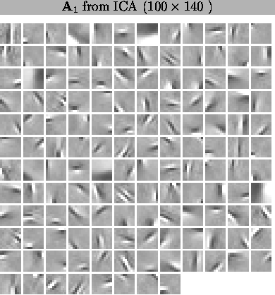
**Figure:** 70 independent components and the same as negative versions are used as the initialisation of $\overline{\mathbf{A}_1}$ . $\overline{\mathbf{B}_{1}}$ is initialised to zero.
$\begin{figure} \begin{center} \begin{tabular}{c} $\mathbf{A}_{1}$\space from ... ...e=pics/img_1_A1.eps,width=0.7\textwidth} \end{tabular} \end{center} \end{figure}$

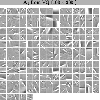
**Figure:** The vector quantisation (VQ) initialisation with 200 model vectors is shown for comparison. There are more vectors that use the whole area since VQ yields a maximally sparse representation. VQ does not have the symmetry between light and dark and light features are clearly dominating.
$\begin{figure} \begin{center} \begin{tabular}{c} $\mathbf{A}_{1}$\space from ... ...ile=pics/img_vq.eps,width=0.7\textwidth} \end{tabular} \end{center} \end{figure}$

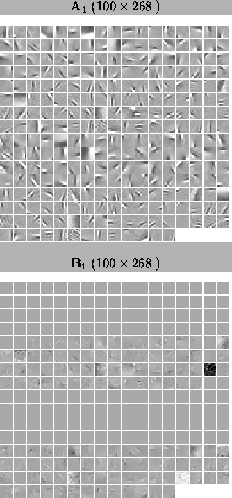
**Figure:** After 100 sweeps through the data. The reconstruction error of s₁ and u₁ are used as data for another run on ICA to get more basis vectors. Now the matrix $\overline{\mathbf{B}_{1}}$ has nonzero entries, too.
$\begin{figure} \begin{center} \begin{tabular}{c} $\mathbf{A}_{1}$\space ($100... ...pics/img_101_B1.eps,width=0.6\textwidth} \end{tabular} \end{center} \end{figure}$

The sources were updated for one hundred sweeps and the least useful ones were removed. Now the second layer had 210 neurons. The sources were updated until sweep 500 when the sources s₂ and variance sources u₂ of the second layer were fed to ICA once again to get initial values for A₂ and B₂ in Figure

. The new sources on the third layer were updated for 200 sweeps and during that the second layer sources were updated every fifth sweep.

The sources on the second layer are ordered for visualisation purposes based on the connections from the third layer. Each dimension of the means of the weights A₂ and B₂ are scaled to zero mean and unit variance and fed to the self-organising map (SOM) [39]. The patches are then organised close to their best matching unit in the SOM.

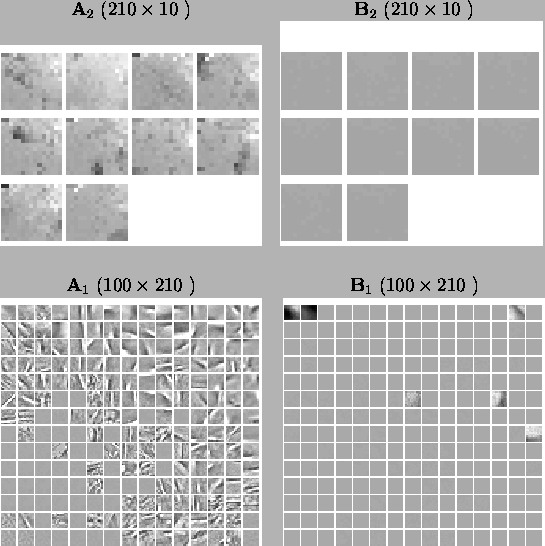
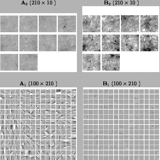
**Figure:** After 500 sweeps through the data. The least useful sources have been pruned away. The sources of the second layer s₂ and u₂ are fed to ICA to get initial values for A₂ and B₂. The sources have been ordered based on A₂ and B₂. The ten patches in A₂ and B₂ correspond to the ten sources on the third layer. The pixels of A₂ and B₂ correspond to the 210 sources on the second layer and thus to the patches of A₁ and B₁.
$\begin{figure} \begin{tabular}{cc} $\mathbf{A}_{2}$\space ($210 \times 10$ ) &... ...epsfig{file=pics/img_501_B1.eps,width=0.47\textwidth} \end{tabular} \end{figure}$

Next, also the weights were released to be updated. The second layer was ``kept alive'' for 1500 sweeps. Figure

shows the situation at sweep 1000. The algorithm has simplified the model by killing neurons. The ``dead'' neurons are removed and everything is updated without using the special states until finally at sweep 6000 the final results are shown in Figure

**Figure:** At sweep 1000. After releasing the weights the algorithm has started to simplify the model. Dead neurons can be seen in the lower left corner of A₁. The patches in B₁ are either clearly close to zero or clearly differ from zero. The emphasis on the second layer has moved from B₂ to A₂.
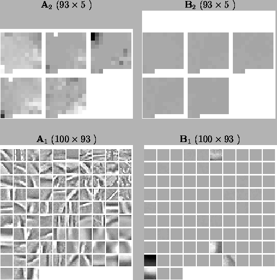
$\begin{figure} \begin{tabular}{cc} $\mathbf{A}_{2}$\space ($210 \times 10$ ) &... ...psfig{file=pics/img_1000_B1.eps,width=0.47\textwidth} \end{tabular} \end{figure}$

**Figure:** Results at sweep 6000. ``Dead'' neurons have been removed.
$\begin{figure} \begin{tabular}{cc} $\mathbf{A}_{2}$\space ($93 \times 5$ ) & $... ...{file=pics/img_6000_B1.eps,width=0.47\textwidth} \end{tabular} \par\end{figure}$