Variational Bayesian learning

In Bayesian data analysis and estimation methods MacKay03, Gelman95,Jordan99,Neal96, all the uncertain quantities are modelled in terms of their joint probability density function (pdf). The key principle is to construct the joint posterior pdf for all the unknown quantities in a model, given the data sample. This posterior density contains all the relevant information on the unknown variables and parameters.

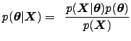
Denote by $\boldsymbol{\theta}$ the set of all model parameters and other unknown variables that we wish to estimate from a given data set $\boldsymbol{X}$. The posterior probability density $p(\boldsymbol{\theta}\vert \boldsymbol{X})$ of the parameters $\boldsymbol{\theta}$ given the data $\boldsymbol{X}$ is obtained from Bayes rule¹

$$p(\boldsymbol{\theta}\vert \boldsymbol{X}) = \hspace{2mm} \frac{ ... ...ymbol{X}\vert \boldsymbol{\theta}) p(\boldsymbol{\theta})}{ p(\boldsymbol{X}) }$$ (1)

Here $p( \boldsymbol{X}\vert \boldsymbol{\theta})$ is the likelihood of the parameters $\boldsymbol{\theta}$ given the data $\boldsymbol{X}$, $p(\boldsymbol{\theta})$ is the prior pdf of these parameters, and

$$p( \boldsymbol{X}) = \hspace{2mm} \int_{\boldsymbol{\theta}} p( \... ...symbol{X}\vert \boldsymbol{\theta}) p(\boldsymbol{\theta}) d\boldsymbol{\theta}$$ (2)

is a normalising term which is called the evidence. The evidence can be directly understood as the marginal probability of the observed data $\boldsymbol{X}$ assuming the chosen model ${\cal H}$. By evaluating the evidences $p(\boldsymbol{X})$ for different models ${\cal H}_i$, one can therefore choose the model which describes the observed data with the highest probability² Bishop95, MacKay03.

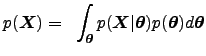
Variational Bayesian learning Barber98NNML,Hinton93COLT,Lappal-Miskin00,MacKay95Ens,MacKay03 is a fairly recently introduced Hinton93COLT,MacKay95Ens approximate fully Bayesian method, which has become popular because of its good properties. Its key idea is to approximate the exact posterior distribution $p(\boldsymbol{\theta}\vert \boldsymbol{X})$ by another distribution $q(\boldsymbol{\theta})$ that is computationally easier to handle. The approximating distribution is usually chosen to be a product of several independent distributions, one for each parameter or a set of similar parameters.

Variational Bayesian learning employs the Kullback-Leibler (KL) information (divergence) between two probability distributions $q(v)$ and $p(v)$. The KL information is defined by the cost function Haykin98

$${\cal J}_{\mathrm{KL}}(q \parallel p) = \hspace{1mm} \int_v q(v) \ln \frac{q(v)}{p(v)} dv$$ (3)

which measures the difference in the probability mass between the densities $q(v)$ and $p(v)$. Its minimum value 0 is achieved when the densities $q(v)$ and $p(v)$ are the same.

The KL information is used to minimise the misfit between the actual posterior pdf $p(\boldsymbol{\theta}\vert \boldsymbol{X})$ and its parametric approximation $q(\boldsymbol{\theta})$. However, the exact KL information ${\cal J}_{\mathrm{KL}}(q(\boldsymbol{\theta}) \parallel p(\boldsymbol{\theta}\vert \boldsymbol{X}))$ between these two densities does not yet yield a practical cost function, because the normalising term $p(\boldsymbol{X})$ needed in computing $p(\boldsymbol{\theta}\vert \boldsymbol{X})$ cannot usually be evaluated.

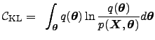
Therefore, the cost function used in variational Bayesian learning is defined Hinton93COLT,MacKay95Ens

$${\cal C}_{\mathrm{KL}}= {\cal J}_{\mathrm{KL}}(q(\boldsymbol{\theta}) \parallel p(\boldsymbol{\theta}\vert \boldsymbol{X})) - \ln p(\boldsymbol{X})$$ (4)

After slight manipulation, this yields

$${\cal C}_{\mathrm{KL}}= \hspace{2mm} \int_{\boldsymbol{\theta}} q... ...ldsymbol{\theta})}{ p(\boldsymbol{X},\boldsymbol{\theta})} d\boldsymbol{\theta}$$ (5)

which does not require $p(\boldsymbol{X})$ any more. The cost function ${\cal C}_{\mathrm{KL}}$ consists of two parts:

$${\cal C}_q= \left< \ln q(\boldsymbol{\theta}) \right> = \hspace{2... ...\theta}} q(\boldsymbol{\theta}) \ln q(\boldsymbol{\theta}) d\boldsymbol{\theta}$$ (6)

$${\cal C}_p= \left< - \ln p(\boldsymbol{X},\boldsymbol{\theta}) \r... ...dsymbol{\theta}) \ln p(\boldsymbol{X},\boldsymbol{\theta}) d\boldsymbol{\theta}$$ (7)

where the shorthand notation $\left< \cdot \right>$ denotes expectation with respect to the approximate pdf $q(\boldsymbol{\theta})$.

In addition, the cost function ${\cal C}_{\mathrm{KL}}$ provides a bound for the evidence $p(\boldsymbol{X})$. Since ${\cal J}_{\mathrm{KL}}(q \parallel p)$ is always nonnegative, it follows directly from (4) that

$${\cal C}_{\mathrm{KL}}\geq - \ln p(\boldsymbol{X})$$ (8)

This shows that the negative of the cost function bounds the log-evidence from below.

It is worth noting that variational Bayesian ensemble learning can be derived from information-theoretic minimum description length coding as well Hinton93COLT. Further considerations on such arguments, helping to understand several common problems and certain aspects of learning, have been presented in a recent paper Honkela04TNN.

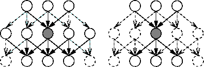
The dependency structure between the parameters in our method is the same as in Bayesian networks Pearl88. Variables are seen as nodes of a graph. Each variable is conditioned by its parents. The difficult part in the cost function is the expectation $\left< \ln p(\boldsymbol{X},\boldsymbol{\theta}) \right>$ which is computed over the approximation $q(\boldsymbol{\theta})$ of the posterior pdf. The logarithm splits the product of simple terms into a sum. If each of the simple terms can be computed in constant time, the overall computational complexity is linear.

In general, the computation time is constant if the parents are independent in the posterior pdf approximation $q(\boldsymbol{\theta})$. This condition is satisfied if the joint distribution of the parents in $q(\boldsymbol{\theta})$ decouples into the product of the approximate distributions of the parents. That is, each term in $q(\boldsymbol{\theta})$ depending on the parents depends only on one parent. The independence requirement is violated if any variable receives inputs from a latent variable through multiple paths or from two latent variables which are dependent in $q(\boldsymbol{\theta})$, having a non-factorisable joint distribution there. Figure 1 illustrates the flow of information in the network in these two qualitatively different cases.

Figure 1: The dash-lined nodes and connections can be ignored while updating the shadowed node. Left: In general, the whole Markov blanket needs to be considered. Right: A completely factorial posterior approximation with no multiple computational paths leads to a decoupled problem. The nodes can be updated locally.

Our choice for $q(\boldsymbol{\theta})$ is a multivariate Gaussian density with a diagonal covariance matrix. Even this crude approximation is adequate for finding the region where the mass of the actual posterior density is concentrated. The mean values of the components of the Gaussian approximation provide reasonably good point estimates of the corresponding parameters or variables, and the respective variances measure the reliability of these estimates. However, occasionally the diagonal Gaussian approximation can be too crude. This problem has been considered in context with independent component analysis in Ilin03ICA, giving means to remedy the situation.

Taking into account posterior dependencies makes the posterior pdf approximation $q(\boldsymbol{\theta})$ more accurate, but also usually increases the computational load significantly. We have earlier considered networks with multiple computational paths in several papers, for example Lappalainen00,Valpola02IJCNN,Valpola02NC,Valpola03IEICE. The computational load of variational Bayesian learning then becomes roughly quadratically proportional to the number of unknown variables in the MLP network model used in Lappalainen00,Valpola03IEICE,Honkela05NIPS.

The building blocks (nodes) introduced in this paper together with associated structural constraints provide effective means for combating the drawbacks mentioned above. Using them, updating at each node takes place locally with no multiple paths. As a result, the computational load scales linearly with the number of estimated quantities. The cost function and the learning formulas for the unknown quantities to be estimated can be evaluated automatically once a specific model has been selected, that is, after the connections between the blocks used in the model have been fixed. This is a very important advantage of the proposed block approach.