Linear dynamic models for the sources and variances

Sometimes it is useful to complement the linear factor analysis model

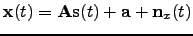$${\bf x}(t) = {\bf As}(t) + {\mathbf{a}} + {\bf n}_x(t)$$ (45)

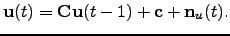
with a recursive one-step prediction model for the source vector ${\bf s}(t)$:

$${\mathbf{s}}(t) = {\mathbf{B}}{\mathbf{s}}(t-1) + {\mathbf{b}} + {\mathbf{n}}_s(t)$$ (46)

The noise term ${\mathbf{n}}_s(t)$ is called the innovation process. The dynamic model of the type (45), (46) is used for example in Kalman filtering Haykin98,Haykin01Kalman, but other estimation algorithms can be applied as well Haykin98. The left subfigure in Fig. 7 depicts the structure arising from Eqs. (45) and (46), built from the blocks.

Figure 7: Three model structures. A linear Gaussian state-space model (left); the same model complemented with a super-Gaussian innovation process for the sources (middle); and a dynamic model for the variances of the sources which also have a recurrent dynamic model (right).

[width=0.146]kalman [width=0.27]srcdyn [width=0.324]vardyn

A straightforward extension is to use variance sources for the sources to make the innovation process super-Gaussian. The variance signal ${\mathbf{u}}(t)$ characterises the innovation process of ${\mathbf{s}}(t)$, in effect telling how much the signal differs from the predicted one but not in which direction it is changing. The graphical model of this extension is depicted in the middle subfigure of Fig. 7. The mathematical equations describing this model can be written in a similar manner as for the hierarchical variance models in the previous subsection.

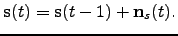
Another extension is to model the variance sources dynamically by using one-step recursive prediction model for them:

$${\mathbf{u}}(t) = {\mathbf{C}}{\mathbf{u}}(t-1) + {\mathbf{c}} + {\mathbf{n}}_u(t).$$ (47)

This model is depicted graphically in the rightmost subfigure of Fig. 7. In context with it, we use the simplest possible identity dynamical mapping for ${\mathbf{s}}(t)$:

$${\mathbf{s}}(t) = {\mathbf{s}}(t-1) + {\mathbf{n}}_s(t).$$ (48)

The latter two models introduced in this subsection will be tested experimentally later on in this paper.