Nonlinear relational Markov networks

Bayesian networks assume acyclicity of the network structure. The directed edges in the graph can be interpreted as causal dependencies and nothing can cause itself. The same assumption is inherited by BLPs and PRMs.^6.1 In some cases it is difficult or irrelevant to try to model the direction of the dependency. Say, whether the husband adopts opinions from his wife, or vice versa, or whether people with certain combinations of opinions are more likely to marry. Using directed edges for describing friendship would definitely lead into cycles with a group of friends. Markov networks (see Section 3.1.2) model dependencies with undirected edges so that it only tells that there is a dependency but not what causes what.

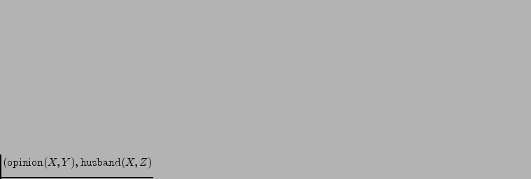
Relational Markov networks (RMN) by Taskar et al. (2002) are to Markov networks what BLPs are to Bayes networks. A RMN is specified by a set of clique templates (the logical part) and a potential for each clique template (the probabilistic part). For instance, the probabilistic part of the template $(\mathrm{opinion}(X,Y), \mathrm{husband}(X,Z)$, $\mathrm{opinion}(Z,Y))$ could describe how the opinions of the husband $X$ and wife $Z$ about the wine $Y$ are related. Given a relational database, the RMN produces an unrolled Markov network over all the attributes in the data. The cliques instantiated by a certain template share the same clique potential. Note that an RMN does not require explicit combination rules.

The general inference task in RMNs is to compute the posterior distribution over all the attributes. The network induced by data can be very large and densely connected, so exact inference is often intractable. The loopy belief propagation algorithm by Murphy et al. (1999) (see Section 3.1.1) is used as an approximation. The learning task, or the estimation of the clique potentials, requires alternating between updating the parameters of the potentials and running the inference algorithm on the unrolled Markov network.

Nonlinear relational Markov networks (NRMN), introduced in Publication VI, combine the ideas of relational Markov networks by Taskar et al. (2002) and nonlinear Markov networks (NMN) by Hofmann and Tresp (1998) (see Section 3.1.2). The combination is not very straightforward because the models are quite different: RMN specifies potentials over cliques of the network whereas NMN specifies a distribution of each variable given its neighbours in the network. In NRMN, the first approach is chosen.

Recall Figure 3.1 that shows a Markov network and its join tree. A node in the join tree corresponds to a clique in a Markov network. NRMN defines a probability distribution over the attributes in each clique template. The distributions are provided by HNFA described in Section 4.4.2. The maximum entropy combination rule requires marginalisation of probability distributions. In nonlinear models, this cannot usually be done exactly and therefore another combination rule was selected. In the product-of-experts (PoE) combination rule, the probability density is the average of the incoming probability densities on the logarithmic scale. A characteristic of PoE is that implicit weighting happens in some sense automatically. When one of the experts gives a distribution with high entropy (little information) and another one with low entropy (much information), the combination is close to the latter one.

NRMNs extend graphical models in both nonlinear and relational directions at the same time. Convergence is guaranteed regardless of loops, unlike in the loopy BP algorithm. There is a lot of room for improvement, though. The current version of NRMN includes many simplifying assumptions, such as diagonality of the posterior covariance matrix in HNFA, and separate learning of experts. Experiments with the game of Go (see Figure 6.5) give promise for NRMNs.

Figure 6.5: Top left: The board of a Go game in progress. Two players alternately place stones on empty points trying to surround area and opponent stones. Top right: The expected owner of each point is visualised with the shade of grey. For instance, the two white stones in the upper right corner are very likely to be captured. Bottom left: The strings of stones with their expected owner as the colour of the square. Pairs of related strings are connected with a blue line if the blocks have same colours and with a red line when the blocks have opposing colours. The lines also represent the structure of the implied Markov network. Bottom right: The covariance between owning a point and scoring high can be used to determine which parts of the board are important (red). The study of this kind of data is left as future work.