Hierarchical nonlinear factor analysis

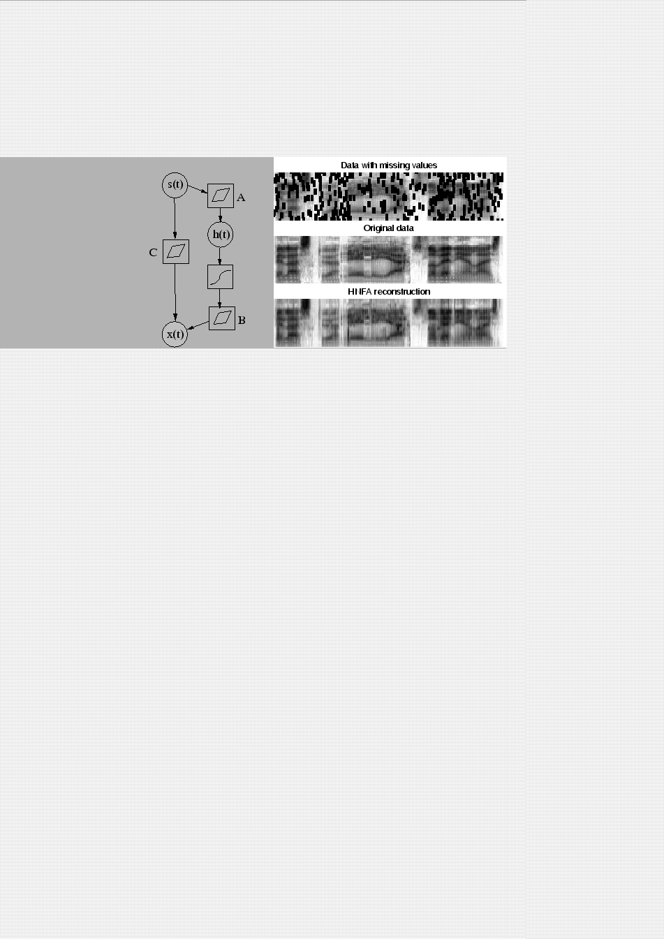
In hierarchical nonlinear factor analysis (HNFA) (Raiko, 2001; Valpola et al., 2003b), there are a number of layers of Gaussian variables, the bottom-most layer corresponding to the data. There is a linear mixture mapping from each layer to all the layers below it. The middle layer variables are immediately followed by a nonlinearity. The model structure for a three-layer network using Bayes Blocks is depicted in the left subfigure of Figure 4.6. Model equations are

$$\mathbf{h}(t) = \mathbf{A}\mathbf{s}(t) + \mathbf{a} + \mathbf{n}_h(t)$$ (4.18)

$$\mathbf{x}(t) = \mathbf{B}\boldsymbol{\phi}[ \mathbf{h}(t) ] + \mathbf{C}\mathbf{s}(t) + \mathbf{b} + \mathbf{n}_x(t) \, ,$$ (4.19)

where $\mathbf{n}_h(t)$ and $\mathbf{n}_x(t)$ are Gaussian noise terms and the nonlinearity $\phi(\xi) = \exp(-\xi^2)$ operates on each element of its argument vector separately. This activation function has the universal approximation property as well (see Stinchcombe and White, 1989, for proof). Note that the short-cut mapping ${\bf C}$ from sources to observations means that hidden nodes only need to model the deviations from linearity.

Figure 4.6: Left: The model structure for hierarchical nonlinear factor analysis (HNFA). Right: Some speech data with and without missing values (Setting 1) and the reconstruction given by HNFA.

HNFA has latent variables $\mathbf{h}(t)$ in the middle layer, whereas in nonlinear FA, the middle layer is purely computational. This results in some differences. Firstly, the cost function $\mathcal{C}$ in HNFA is evaluated without resorting to approximation, since the required integrals can be solved analytically. Secondly, the computational complexity of HNFA is linear with respect to the number of sources, whereas the computational complexity of nonlinear FA is quadratic. HNFA is thus applicable to larger problems, and it is feasible to use even more layers than three. Also, the efficient pruning facilities of Bayes Blocks allow determining whether the nonlinearity is really needed and pruning it out when the mixing is linear, as demonstrated by Honkela et al. (2005).

The good properties of HNFA come with a cost. The simplifying assumption of diagonal covariance of the posterior approximation, made both in nonlinear FA and HNFA, is much stronger in HNFA because it applies also in the middle layer variables $\mathbf{h}(t)$. Publication II compares the two methods in reconstructing missing values in speech spectrograms. As seen in the right subfigure of Figure 4.6, HNFA is able to reconstruct the spectrogram reasonably well, but quantitative comparison reveals that the models learned in HNFA are more linear (and thus in some cases worse) compared to the ones learned in nonlinear FA.