Nonlinear factor analysis

Recall factor analysis described in Section 3.1.3, in which the conditional density in Equation (3.14) is restricted to be linear. In nonlinear FA, the generative mapping from factors (or latent variables or sources) to data is no longer restricted to be linear. The general form of the model is

$${\bf x}(t) = {\bf f}({\bf s}(t), \boldsymbol{\theta}_f) + {\bf n}(t) \, .$$ (4.6)

This can be viewed as a model about how the observations were generated from the sources. The vectors ${\bf x}(t)$ are observations at time $t$, ${\bf s}(t)$ are the sources, and ${\bf n}(t)$ are noise. The function ${\bf f}(\cdot)$ is a mapping from source space to observation space parametrised by $\boldsymbol{\theta}_f$.

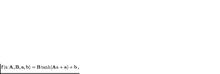
Lappalainen and Honkela (2000) use a multi-layer perceptron (MLP) network (see Haykin, 1999) with tanh-nonlinearities to model the mapping ${\bf f}$:

$${\bf f}({\bf s}; {\bf A}, {\bf B}, {\bf a}, {\bf b}) = {\bf B}\tanh({\bf A}{\bf s} + {\bf a}) + {\bf b} \, ,$$ (4.7)

where the $\tanh$ nonlinearity operates on each component of the input vector separately. The mapping ${\bf f}$ is thus parameterised by the matrices ${\bf A}$ and ${\bf B}$ and bias vectors ${\bf a}$ and ${\bf b}$. MLP networks are well suited for nonlinear FA. First, they are universal function approximators (see Hornik et al., 1989, for proof) which means that any type of nonlinearity can be modelled by them in principle. Second, it is easy to model smooth, nearly linear mappings with them. This makes it possible to learn high dimensional nonlinear representations in practice.

The traditional use of MLP networks differs a lot from the use in nonlinear FA. Traditionally MLP networks are used in a supervised manner, mapping known inputs $\mathbf{s}(t)$ to desired outputs $\mathbf{x}(t)$. During training of the network, both $\mathbf{s}(t)$ and $\mathbf{x}(t)$ are observed, whereas in nonlinear FA, $\mathbf{s}(t)$ is always latent. The traditional learning problem is much easier and can be reasonably solved by using just point estimates.

The used posterior approximation is a fully factorial Gaussian:

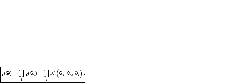$$q(\boldsymbol{\Theta}) = \prod_i q(\Theta_i) = \prod_i \mathcal{N}\left(\Theta_i;\overline{\Theta}_i,\widetilde{\Theta}_i\right),$$ (4.8)

where the unknown variables $\Theta_i$ include the factors $\mathbf{s}$, the matrices $\mathbf{A}$ and $\mathbf{B}$, and other parameters. Thus for each unknown variable $\theta_i$, there are two parameters, the posterior mean $\overline{\Theta}_i$ and the posterior variance $\widetilde{\Theta}_i$. The distribution that propagates through the nonlinear mapping $\mathbf{f}$ has to be approximated. Honkela and Valpola (2005) suggest to do this by linearising the tanh-nonlinearities using a Gauss-Hermite quadrature. This works better than a Taylor approximation or using a Gauss-Hermite quadrature on the whole mapping $\mathbf{f}$.

Using linear independent component analysis (ICA, see Section 3.1.4) on sources $\mathbf{s}(t)$ found by nonlinear factor analysis is a solution to the nonlinear ICA problem, that is, finding independent components that have been nonlinearly mixed to form the observations. A variety of approaches for nonlinear ICA are reviewed by Jutten and Karhunen (2004). Often, a special case known as post-nonlinear ICA is considered. In post-nonlinear ICA, the sources are linearly mixed with the mapping $\mathbf{A}$ followed by component-wise nonlinear functions:

$${\bf f}({\bf s}; \boldsymbol{\theta}_f) = \boldsymbol{\phi}({\bf A}{\bf s} + {\bf a}),$$ (4.9)

where the nonlinearity $\boldsymbol{\phi}$ again operates on each element of its argument vector separately. Ilin and Honkela (2004) consider post-nonlinear ICA by variational Bayesian learning.