Factor analysis and principal component analysis

Factor analysis (Hyvärinen et al., 2001; Harman, 1967; Kendall, 1975) (FA) can be seen as a Bayesian network consisting of two layers, depicted in Figure 3.2. The top layer contains latent variables $\mathbf{s}(t)$ and the bottom layer contains observations $\mathbf{x}(t)$. The two layers are fully connected, that is, each observation has all of the latent variables as its parents. The index $t$ stands for the data case.

Figure: Graphical representations of factor analysis, principal component analysis, and independent component analysis are the same. Latent variables in the top layer are fully connected to the observations in the bottom layer. In this case, the vectors $\mathbf{s}(t)$ are two dimensional and $\mathbf{x}(t)$ are three dimensional.

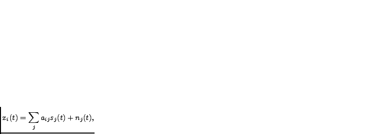
The mapping from factors to data is linear^3.2

$$\mathbf{x}(t) = \mathbf{A}\mathbf{s}(t) + \mathbf{n}(t),$$ (3.13)

or componentwise

$$x_i(t) = \sum_j a_{ij} s_j(t) + n_j(t),$$ (3.14)

where $\mathbf{n}(t)$ is noise or reconstruction error vector. Typically the dimensionality of the factors is smaller than that of the data. Factors and noise are assumed to have a Gaussian distribution with an identity and diagonal covariance matrix, respectively. Recalling the notation from Section 2.3, parameters $\boldsymbol{\theta}$ include the weight matrix $\mathbf{A}$ and noise covariance for $\mathbf{n}(t)$.

Equation (3.14) does not fix the matrix $\mathbf{A}$, since there is a group of rotations that yields identical observation distributions. Several criteria have been suggested for determining the rotation. One is parsimony, which roughly means that most of the values in $\mathbf{A}$ are close to zero. Another one leads to independent component analysis described in Section 3.1.4. Sections 4.2 and 4.4.2 describe extensions of factor analysis releasing from the linearity assumption of the dependency between factors and observations.

Principal component analysis (PCA) (Jolliffe, 1986; Hyvärinen et al., 2001; Kendall, 1975), equivalent to the Hotelling transform, the Karhunen-Loève transform, and the singular value decomposition, is a widely used method for finding the most important directions in the data in the mean-square sense. It is the solution of the FA problem under low noise (see Bishop, 2006) with orthogonal principal components (the columns of the weight matrix $\mathbf{A}$).

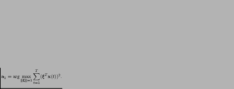
The first principal component $\mathbf{a}_1$ corresponds to the line on which the projection of the data has the greatest variance:

$$\mathbf{a}_1 = \arg \max_{\vert\vert\boldsymbol{\xi}\vert\vert=1} \sum_{t=1}^T(\boldsymbol{\xi}^T\mathbf{x}(t))^2.$$ (3.15)

The other components are found recursively by first removing the projections to the previous principal components:

$$\mathbf{a}_k = \arg \max_{\vert\vert\boldsymbol{\xi}\vert\vert=1}... ...}(t)-\sum_{i=1}^{k-1}\mathbf{a}_i \mathbf{a}_i^T \mathbf{x}(t)\right)\right]^2.$$ (3.16)

There are many other ways to formulate PCA, including probabilistic PCA (Bishop, 1999). In practice, the principal components are found by calculating the eigenvectors of the covariance matrix $\mathbf{C}$ of the data

$$\mathbf{C} = E\left\{ \mathbf{x}(t)\mathbf{x}(t)^T \right\}$$ (3.17)

The eigenvalues are positive and they correspond to the variances of the projections of data on the eigenvectors. The weight matrix $\mathbf{A}$ is formed from the eigenvectors and it is always orthogonal.