Nonlinear state-space models

In many cases, measurements originate from a dynamical system and form time series. In such cases, it is often useful to model the dynamics in addition to the instantaneous observations. Valpola and Karhunen (2002) extend the nonlinear factor analysis model by adding a nonlinear model for the dynamics of the sources ${\bf s}(t)$. This results in a state-space model where the sources can be interpreted as the internal state of the underlying generative process. On the other hand, nonlinear state-space models are a direct extension of linear state-space models (see Section 3.1.6) where the linearity assumption is relaxed.

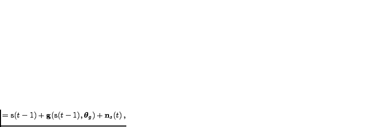
The nonlinear static model of Equation (4.6) is extended by adding another nonlinear mapping $\mathbf{g}$ to model the dynamics. This leads to source model

$${\bf s}(t) = {\bf s}(t-1) + {\bf g}({\bf s}(t-1), \boldsymbol{\theta}_g) + {\bf n}_s(t) \, ,$$ (4.10)

$${\bf g}({\bf s}; {\bf C}, {\bf D}, {\bf c}, {\bf d}) = {\bf D}\tanh({\bf C}{\bf s} + {\bf c}) + {\bf d} \, ,$$ (4.11)

where ${\bf s}(t)$ are the sources (states), ${\bf n}_s(t)$ is the Gaussian noise, and the dynamics mapping ${\bf g}(\cdot)$ is modelled by an MLP network.

In case the dynamic system is changing slowly, there are high correlations between consecutive states. This is taken into account by giving up the fully factorial posterior approximation used in nonlinear FA. The posterior distribution of each component $i$ of the state vector $\mathbf{s}(t)$ is conditioned on the same component $i$ of the state vector $\mathbf{s}(t-1)$. The approximate density $q(s_i(t)\mid s_i(t-1))$ is parameterised by the mean, linear dependence, and variance (see Valpola and Karhunen, 2002, for details).

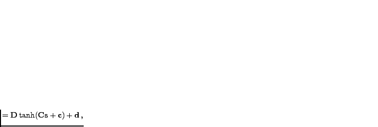
Considering the sequence of consecutive mappings $\mathbf{g}$ in the system dynamics, where each mapping $\mathbf{g}$ consists of a linear mapping, component-wise nonlinearities, and a second linear mapping, one might think that one of the two linear mappings before and after the states is redundant since two consecutive linear mappings can always be combined into one. The second mapping allows the model to select a representation where the variational approximation is most accurate. It also allows the dimensionality of the state-space to be different from the number of used nonlinearities, thus decreasing computational complexity in some cases.

An important advantage of the VB method is its ability to learn a high-dimensional latent source space. Computational and over-fitting problems have been major obstacles in developing this kind of unsupervised methods thus far. Potential applications for the method include prediction and process monitoring, control, and speech enhancement for recognition. Is process monitoring, Ilin et al. (2004) show that VB learning is able to find a model which is capable of detecting an abrupt change in the underlying dynamics of a fairly complex nonlinear process.