Nonlinear Relational Markov Networks (NRMN)

In nonlinear relational Markov networks (NRMN), the clique potentials are replaced by a probability density function for continuous values, in this case HNFAThe combination of these two methods is not completely straightforward. For instance, marginalisation required by the BP algorithm is often difficult with nonlinear models. Also, algorithmic complexity needs to be considered, since the model will be quite demanding. One of the key points is to use probability densities $p$ in place of potentials $\boldsymbol{\Phi}$. Then, overlapping templates give multiple probability functions for some variable and they are combined using the product-of-experts combination rule described below.

Combination Rules: One of the non-trivialities in making relational extensions of probabilistic models is the so called combination rule [7]. When the structure of the graphical model is determined by the data, one cannot know in advance how many links there are for each node. One solution is to use combination rules such as the noisy-or. Combination rule transforms a number of probability functions into one. Noisy-or does not generalise well to continuous values, but two alternatives are introduced below.

Using a Markov network and the BP algorithm corresponds to using probability densities as potentials and the maximum entropy combination rule. The probability densities $p_C({\mathbf{x}}(C))$ are combined to form the joint probability distribution by maximising the entropy of $p(\boldsymbol{X})$ given that all instantiations of $p_C({\mathbf{x}}(C))$ coalesce with the corresponding marginals of $p(\boldsymbol{X})$. For singly connected networks, this means that the joint distribution is $p(\boldsymbol{X}) = \prod_c p_c({\mathbf{x}}(c)) / \prod_k p_k({\mathbf{x}}(k))$, where $k$ runs over pairs of instantiations of templates and ${\mathbf{x}}(k)$ contains the shared attributes in those pairs. Marginalisation of nonlinear models cannot usually be done exactly and therefore one should be very careful with the denominator. Also, one should take care in handling loops.

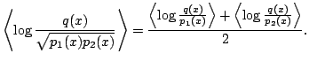
In the product-of-experts (PoE) combination rule, the logarithm of the probability density of each variable is the average of the logarithms of the probability functions that the variable is included in: $p(x) \propto \sqrt[n]{\prod_{C \in {\mathbf{C}}} \prod_{c \in C(\mathcal{I})} p_C(x)}$ for all $x \in \boldsymbol{X}$, where only those $n$ instantiated templates $c$ that contain $x$, are considered. PoE is easy to implement in the variational Bayesian framework because the term in the cost function (3) can be split into familiar looking terms. Consider the combination of two probability functions $p_1(x)$ and $p_2(x)$ (that are assumed to be independent):

$$\left< \log \frac{q(x)}{\sqrt{p_1(x) p_2(x)}} \right> = \frac{\le... ...\log \frac{q(x)}{p_1(x)} \right> + \left< \log \frac{q(x)}{p_2(x)} \right>}{2}.$$ (4)

A characteristic of PoE is that implicit weighting happens in some sense automatically. When one of the experts gives a distribution with a large variance and another one with a small variance, the combination is close to the one with small variance.

Inference in Loopy Networks: Inferring unobserved attributes in a database is in this case an iterative process which should end up in a cohesive whole. Information can traverse through multiple relations. The basic element in the inference algorithm of Bayes Blocks is the update of the posterior approximation $q(\cdot)$ of a single unknown variable, assuming the rest of the distribution fixed. The update is done such that the cost function (3) is minimised. One should note that when the distribution over the Markov blanket of a variable is fixed, the local update rules apply, regardless of any loops in the network. Therefore the use of local update rules is well founded, that is, local inference in a loopy network does not bring any additional heuristicity to the system. Also, since the inference is based on minimising a cost function, the convergence is guaranteed, unlike in the BP algorithm.

Learning: The learning or parameter estimation problem is to find the probability functions associated with the given clique templates ${\mathbf{C}}$. Now that we use probability functions instead of potentials, it is possible in some cases to separate the learning problem into parts. For each template $C \in {\mathbf{C}}$, find the appropriate instantiations $c \in C(\mathcal{I})$ and collect the associated attributes ${\mathbf{x}}(c)$ into a table. Learn a HNFA model for this table ignoring the underlying relations. This divide-and-conquer strategy makes learning comparatively fast, because all the interaction is avoided. There are some cases that forbid this. If the data contains missing values, they need to be inferred using the method in the previous paragraph. Also, it is possible to train experts cooperatively rather than separately [3].

Clique Templates: In data mining, so called frequent sets are often mined from binary data. Frequent sets are groups of binary variables that get the value $1$ together often enough to be called frequent. The generalisation of this concept to continuous values could be called the interesting sets. An interesting set contains variables that have such strong mutual dependencies that the whole is considered interesting. The methodology of inductive logic programming could be applied to finding interesting clique templates. The definition of a measure for interestingness is left as future work. Note that the divide-and-conquer strategy described in the previous paragraph becomes even more important if one needs to consider different sets of templates. One can either learn a model for each template separately and then try combinations with the learned models, or try a combination of templates and learn cooperatively the models for them. Naturally the number of templates is much smaller than the number of combinations and thus the first option is computationally much cheaper.

So what are meaningful candidates for clique templates? For instance, the template $(\mathrm{con}(A), \mathrm{con}(B))$ does not make much sense. Variables $A$ and $B$ are not related to each other, so when all pairs are considered, $\mathrm{con}(A)$ and $\mathrm{con}(B)$ are always independent and thus uninteresting by definition. In general, a template is uninteresting, if it can be split into two parts that do not share any variables. When considering large templates, the number of involved attributes grows large as well, which makes learning more involved. An interesting possibility is to make a hierarchical model. When a large template contains others as subtemplates, one can use the factors ${\mathbf{s}}$ in Eq. (1, 2) of the subtemplate as the attributes for the large template. The factors already capture the internal structure of the subtemplates and thus the probabilistic model of the large template needs only to concentrate on the structure between its subtemplates.