In (linear) factor analysis, continuous valued observation
vectors
![]() are generated from unknown factors (or sources)
are generated from unknown factors (or sources)
![]() , a bias vector
, a bias vector
![]() , and noise
, and noise
![]() by
by
![]() .
The factors and noise are assumed to be Gaussian and independent. The
index
.
The factors and noise are assumed to be Gaussian and independent. The
index ![]() may represent time or the object of the observation. The
mapping
may represent time or the object of the observation. The
mapping
![]() , the factors, and parameters such as the noise
variances are found using Bayesian learning. Factor analysis is close
to principal component analysis (PCA). The unknown factors may
represent some real phenomena, or they may just be auxillary variables
for inducing a dependency between the observations.
, the factors, and parameters such as the noise
variances are found using Bayesian learning. Factor analysis is close
to principal component analysis (PCA). The unknown factors may
represent some real phenomena, or they may just be auxillary variables
for inducing a dependency between the observations.
Hierarchical nonlinear factor analysis (HNFA) [11]
generalises factor analysis by adding more layers of factors
that form a multi-layer perceptron type of a network.
In this paper, there are two layers of factors
![]() and
and
![]() , and the
mappings are:
, and the
mappings are:
The unknown variables
![]() (factors, mappings, and the
parameters) are learned from data with variational Bayesian learning
[4]. A parametric
distribution
(factors, mappings, and the
parameters) are learned from data with variational Bayesian learning
[4]. A parametric
distribution
![]() over the unknown variables
over the unknown variables
![]() is fitted to
the true posterior distribution
is fitted to
the true posterior distribution
![]() where the matrix
where the matrix
![]() contains all the observations
contains all the observations
![]() . The misfit is measured
by Kullback-Leibler divergence
. The misfit is measured
by Kullback-Leibler divergence
![]() . An additional
term
. An additional
term
![]() is included to avoid calculation of the model
evidence term
is included to avoid calculation of the model
evidence term
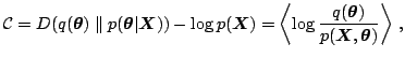
![]() . The cost function is
. The cost function is
It is possible, though slightly impractical, to model also discrete values
in HNFA by using the discrete variable with a soft-max prior
[12]. In the binary case, the ![]() th component of
th component of
![]() is left as a latent auxiliary variable, and an observed
binary variable
is left as a latent auxiliary variable, and an observed
binary variable ![]() is conditioned by
is conditioned by
![]() . The general discrete case
follows analogously requiring more than one auxiliary component of
. The general discrete case
follows analogously requiring more than one auxiliary component of
![]() . The experiments in Section 3 use a thousand copies of a binary
variable having the same conditional probability. They can be united
into one variable by multiplying its cost by one
thousand. Observing 800 ones and 200 zeros corresponds to
fixing the variable to a distribution of 0.8 times one and 0.2 times
zero.
. The experiments in Section 3 use a thousand copies of a binary
variable having the same conditional probability. They can be united
into one variable by multiplying its cost by one
thousand. Observing 800 ones and 200 zeros corresponds to
fixing the variable to a distribution of 0.8 times one and 0.2 times
zero.