Experiments with the Game of Go

Game of Go: Go is an ancient oriental board game. Two players, black and white, alternately place stones on the empty points of the board until they both pass. The standard board is 19 by 19 (i.e. the board has 19 lines by 19 lines), but 13-by-13 and 9-by-9 boards can also be used. The game starts with an empty board and ends when it is divided into black and white areas. The one who has the larger area wins. Stones of one colour form a block when they are 4-connected. Empty points that are 4-connected to a block are called its liberties. When a block loses its last liberty, it is removed from the board. After each move, surrounded opponent blocks are removed and only after that, it is checked whether the block of the played move has liberties or not. There are different rulesets that define more carefully what a ``larger area'' is, whether suicide is legal or not, and how infinite repetitions are forbidden.

Computer Go: Of all games of skill, go is second only to chess in terms of research and programming efforts spent. While go programs have advanced considerably in the last 10-15 years, they can still be beaten easily by human players of moderate skill. [5] One of the reasons behind the difficulty of static board evaluation is the fact that there are stones on board that will eventually be captured, but not in near future. In many cases experienced go players can classify these dead stones with ease, but using a simple look-ahead to determine the status of stones is not always feasible since it might take dozens of moves to actually capture the stones.

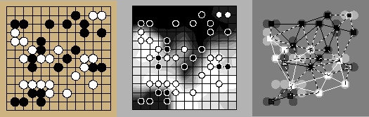
Experiment Setting: The goal of the experiments was to learn to determine the status of the stones without any lookahead. An example situation is given in Figure 2. The data was generated using a go-playing program called Go81 [8] set on level 1 and using randomness to have variability. By playing the game from the current position to the end a thousand times, one gets an estimate of who is going to own each point on the board. Information on the board states was saved to a relational database with two tables for learning an NRMN. The ${\mathbf{x}}(\mathrm{block}(A))$ contains the colour, the number of liberties, the size, distances from the edges, influence features in the spirit of [1], and finally the count of how many times the block survives in the 1000 possible futures. The $\mathrm{ally}(A,B)$ and $\mathrm{enemy}(A,B)$ contain a measure of strength of the connection between the blocks $A$ and $B$ estimated using similar influence features [1]. Only the pairs with a strong enough influence on each other (> 0.02) were included. One thousand 13-by-13 board positions after playing 2 to 60 moves were used for learning.

Two clique templates, $((\mathrm{block}(A),\mathrm{ally}(A,B),\mathrm{block}(B))$ and an analogous one for $\mathrm{enemy}$, were used. HNFA models were taught with 28 attributes of the two blocks and the pair. The dimensionality of the ${\mathbf{s}}$ layer was 8. The learning algorithm pruned the dimensionality of the ${\mathbf{h}}$ layer to 41 for allies and to 47 for enemies. The models were learned for 500 sweeps through the data. A linear factor analysis model was learned with the same data for comparison. A separate collection of 81 board positions with 1576 blocks was used for testing. The status of each block was now hidden from the model and only the other attributes were known. With inference in the network, the status were collectively regressed. As a comparison experiment, the inferences were also done separately, and combined only in the end. Inference required from four to thirty iterations to converge. As a postprocessing step, the regressed survival probabilities $\hat{x}$ were modified with a simple three-parameter function $\hat{x}_\textit{new}=a\hat{x}^b+c$ and the three parameters that gave the smallest error for each setting, were used.

Figure 2: The leftmost subfigure shows the board of a go game in progress. In the middle, the expected owner of each point is visualised with the shade of grey. For instance, the two white stones in the upper right corner are very likely to be captured. The rightmost subfigure shows the blocks with their expected owner as the colour of the square. Pairs of related blocks are connected with a line which is dashed when the blocks are of opposing colours.

Results: The table below shows the root mean square (rms) errors for inferring the survival probabilities of the blocks in test cases. They can be compared to the standard deviation 0.2541 of the probabilities.

rms error	Linear	Nonlinear
Separate regression	0.2172	0.2052
Collective regression	0.2171	0.2037

As expected, nonlinear models were better than linear ones and collective regression was better than separate regression.