The MDHMM training procedure

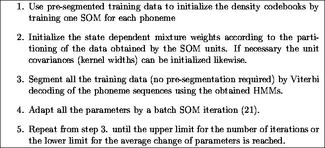
for producing ordered density codebooks and maintaining the ordering throughout the training by the segmental SOM training occurs in the following steps: (This can be compared to Figure 3.)

A batch iteration by the segmental SOM produces new mean vectors $\mbox{\boldmath$\mu$}_{jm}$for Gaussian kernels of mixture density codebook j, by computing the averages of the associated sample vectors $\mbox{\boldmath$O$}_t\:$: 

$$\hat{\mbox{\boldmath$\mu$}}_{jm} = \frac {\sum_{t=1}^{T} \de... ...{\boldmath$O$}_t} {\sum_{t=1}^{T} \delta(q_t,j) h_{o,m} } \:,$$ (20)

where the indicator function $\delta(q_t,j) = 1$, if q_t (the decoded state for time t) is connected to the codebook j (otherwise $\delta(q_t,j) = 0$). In general, each state could use several codebooks and the same codebooks can be connected to several states. Here, the states in the same HMM use the same codebook (see Figure 1). The most probable correct state sequences q corresponding to the observation sequences $\mbox{\boldmath$O$}$are determined by the current segmentation (see Figure 3). The equation (21) is essentially the same as (3). If individual covariance matrices would be needed for each Gaussian kernel, the adaptation formula for $\hat{\mbox{\boldmath$\Sigma$}}_{jm}$corresponding to (21) could be obtained by substituting $\mbox{\boldmath$O$}_t$ in (21) by the matrix of the deviations from the mean vector $(\mbox{\boldmath$O$}_t - \mbox{\boldmath$\mu$}_{jm}) (\mbox{\boldmath$O$}_t - \mbox{\boldmath$\mu$}_{jm})^T$.

The mixture weights that connect individual Gaussian kernels to the output density function of an HMM state (20) are set in the batch iteration to reflect the contribution of the kernels for the output density function of that state:  

$$\hat c_{im} = \frac {\sum_{t=1}^{T} \delta(q_t,i) h_{o,m} } {\sum_{t=1}^{T} [\delta(q_t,i) \sum_{m=1}^{M_i} h_{o,m}]} \:,$$ (21)

where the indicator function $\delta(q_t,i) = 1$, here, if the state q_t = i (otherwise $\delta(q_t,i) = 0$). The neighborhood function h_o,m > 0, if the unit m belongs to the neighborhood of the best-matching unit o of the current codebook (thus h_o,m depends on t via the index o). From the different kinds of neighborhood functions h_o,m [Kohonen, 1995], the simple bubble type is used here for simplicity. After each new adaptation of $\mbox{\boldmath$\mu$}_{jm}$s and c_ims the size of the adaptation neighborhood is decreased gradually until it is empty, and then the process continues by adapting only the parameters of the best-matching mixture for each training sample.