Convergence.

The batch mode is used in the adaptation for faster convergence to acceptable results and easier control of the decrease of the learning rate and the neighborhood. For the training depending on the gradually improving Viterbi segmentation of the data, the batch training is a natural choice to ensure equal weighting of the training words. When the neighborhood is reduced to zero the segmental SOM equals the segmental K-means [Rabiner et al., 1986], which is the conventional ML training algorithm for HMMs.

For the analysis of the convergence of the suggested MDHMM training method mostly the same guidelines are valid as for the segmental K-means [Juang and Rabiner, 1990]. The difference between the segmental K-means and segmental SOM is the same as between the normal K-means [MacQueen, 1967] and the normal batch SOM [Kohonen, 1995] as analyzed in [Luttrell, 1990], for example. If the SOM neighborhood size is small enough to ensure the increase of the likelihood of the model in the parameter adaptation steps the direction of the convergence can be expected to be close to that in the segmental K-means. However, in this HMM training experiments the neighborhood radius of the segmental SOM is gradually decreased to zero and after that only the parameters of the best matching mixture is adapted with steps identical to the segmental K-means.

The models trained by SOM are not optimized to discriminate between different models. LVQ is used for that purpose to optimize the classification boundaries for the areas in the observation sequences, in which the models behave inappropriately, by tuning the density functions (see Section 3.3).

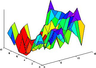
Like the SOM training with zero neighborhood, also the LVQ training forces the codebook to fold and loose its smoothness. The large-scale structure of the codebook is not, however, entirely broken preserving still some potential for smoothing and density approximations. Figure 4 illustrates the breaking of the codebook structure by the zero neighborhood training. The figure shows the values of the mixture Gaussians of a codebook organized into a 14x10 SOM grid for one randomly selected input vector.

  

Figure 4: The responses of the individual mixture density components in the codebook for phoneme /A/ organized into 10x14 grid are plotted for one randomly selected input vector. The first plot (left) is the situation when the radius is decreased to one and the second is after training with zero neighborhood.