Causal structure of the model

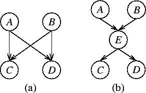
Taking into account causal relations of the environment usually results in simpler and computationally efficient models. Take for example a situation where A and B are known to affect C and D, but the effect is causally mediated through E. If E summarises all the knowledge that A and B have about C and D, then Cand D are conditionally independent of A and B given E. Mathematically this means that

$$P(CD \vert AB) = \sum_i P(CD \vert E_iAB) P(E_i \vert AB) = \sum_i P(CD \vert E_i) P(E_i \vert AB).$$ (23)

It would be possible to consider the situation from the point of view of only the variables A, B, C and D, but then the model would have a dependence from two variables A and B to two variables Cand D. Figure 1 represents graphically the introduction of a mediating variable. The nodes correspond to variables and the arrows denote their causal dependences. Such a graph is called a graphical model [73,59].

  

Figure 1: (a) Graphical representation of the causal structure P(CD | AB). (b) Introduction of a mediating variable E simplifies the structure.

In general, a model with more variables but with simpler dependences is computationally more efficient. Introducing mediating variable Esimplifies the dependences because either only one variable affects two others, as in P(CD | E_i), or two variables affect one, as in P(E_i | AB). This strategy is a second nature to human beings who constantly try to organise the world by splitting complex dependences into simpler ones by introducing hidden, mediating variables, and therefore it is also usually easy to construct models using the same design principle. The mediating variables are not directly observable but can only be inferred from the dependence structure of the observations. These variables are therefore often called hidden or latent variables [25].

From a computational point of view, the efficiency is caused by the fact that the posterior probability of the unknown variables will be a product of many simple terms. Taking the logarithm will then split the product into a sum of many simple terms. Most methods for approximating the posterior probabilities can make use of this property, including the ML and MAP estimators, the EM algorithm, Laplace's method, ensemble learning and many versions of stochastic sampling.