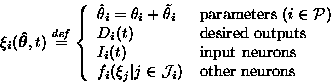
We shall consider a standard MLP-network with input, hidden and output
layers. In order to be able to write the feedforward equations in a
compact form, we shall assign all parameters and outputs of the
neurons a unique index. In our notation, ![]() can mean either the
value of a parameter or output of a neuron, that is,
can mean either the
value of a parameter or output of a neuron, that is, ![]() are used
to denote any value than can be an input for neurons. The set of
indices for the parameters is denoted by
are used
to denote any value than can be an input for neurons. The set of
indices for the parameters is denoted by ![]() and the transfer
functions of the neurons are denoted by fi. The values
and the transfer
functions of the neurons are denoted by fi. The values ![]() are
defined by equation 4.
are
defined by equation 4.
 |
(4) |
For hidden and output neurons the transfer functions fi are like in any conventional neural network. They can be sums of inputs multiplied by weights, sigmoids, radial basis functions, etc.
The cost function for supervised learning is L(MS) + L(DS |
MS) as explained in section 1.1. The description
lengths are computed according to equation 1, with the
exception that the terms ![]() are omitted from L(DS |
MS). For each Di we shall assign a function fj, which is used
to compute the terms
are omitted from L(DS |
MS). For each Di we shall assign a function fj, which is used
to compute the terms ![]() . The set of indices for these
functions is denoted by
. The set of indices for these
functions is denoted by ![]() . Similarly, the set
. Similarly, the set ![]() comprises of the indices of functions fj, which evaluate the terms
comprises of the indices of functions fj, which evaluate the terms
![]() . We can now write down the cost function in terms
of
. We can now write down the cost function in terms
of ![]() and
and ![]() .
.
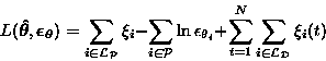 |
(5) |
If a parameter ![]() does not have an associated neuron in the
set
does not have an associated neuron in the
set ![]() , it means that we tacitly assume the probability
distribution
, it means that we tacitly assume the probability
distribution ![]() to be constant throughout the range of
values of
to be constant throughout the range of
values of ![]() , that is, we assume the value of the parameter to
be evenly distributed. It has to be reminded that although the
constant term
, that is, we assume the value of the parameter to
be evenly distributed. It has to be reminded that although the
constant term ![]() can be omitted when adapting the
parameters and their accuracies, it should still be taken into account
when models with different parametrisations are compared.
can be omitted when adapting the
parameters and their accuracies, it should still be taken into account
when models with different parametrisations are compared.
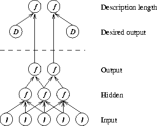 |
The structure of the network is shown in figure 2. Desired outputs are marked by D, input neurons by I, and other neurons by f. The parameters of the network are not shown. The functions f above the dotted line are the ones used to compute the description length of the parameters and the data.