
In practice it is usually impossible to divide the network into orthogonal parts. If the network is topologically ordered, the weight vectors of far-off neurons are usually orthogonal, but adjacent neurons are always nearly parallel. Therefore, it is impossible to make a clear division into functionally separate areas. This does not matter since the algorithm does not make any assumptions about functionally separate areas.
The learning algorithm was tested with artificial data, which has this kind of structure. The data was also sparse, which means that it is possible to represent each sample with only a few models from a large pool of models. Olshausen and Field (1995) have conjectured that natural images have this kind of sparse structure. The data can be seen as a strongly simplified model of the visual input to an amphibian. It's environment is assumed to consist of small insects flying around.
Figure 4.10 (a) shows a sample of the data set. There are supposed to be four insects (we shall call them flies) in arbitrary positions in a wrapped 1-dimensional space. (Wrapped means that when you move in one direction, you eventually come to the same place.) We take an imaginary photograph of the flies, but due to the optics, their images appear blurred. In figure 4.10 (a) one can see only three distinct images. This is because two of the flies happen to be in the nearly same position. Each sample can be described by four models of the flies, if the models correspond to the image of a fly in a given position. Since there are infinitely many positions, there may also be infinitely many models. However, the images of two flies in nearly same positions are very similar, and it is possible to discretise the models without making a large error.
In this test, 40 neurons are used. The learning was done in several parts and for each part the learning parameters were constant (table 4.1). The neurons were organised in a 1-dimensional map and the neighbourhood function was piece-wise linear

Here r is the radius of the neighbourhood. Parameters ![]() and
and ![]() were held constant throughout the learning.
were held constant throughout the learning.
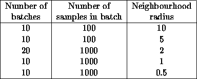
Table 4.1:
Parameters in the test run with artificial data.
The weight vectors learned by the network are presented in figure 4.7. It shows that the network was able to find a sparse representation for the input. Although the flies never occurred alone in the input, each neuron has learned to represent the position of a single fly. The network is topologically ordered: adjacent weight vectors are nearly parallel, while far-off weight vectors are nearly parallel (figure 4.8). Figure 4.9 shows the outputs of the network to inputs with only one fly.
Figure 4.10 shows the outputs to a input with four flies, two of which are in the nearly same position (figure (a)). The projection of the input vector on the weight vectors of the network are shown in figure (b). The competition between neurons with similar weight vectors greatly sharpens the outputs, which are shown in figure (c). The figure clearly shows that the output is a very nonlinear function of the direction of the input vector. Due to the competition between neurons with similar weight vectors the final outputs are much sharper than the projections before competition. On the other hand, neurons with dissimilar weight vectors do not have mutual competition, which allows different parts of the network to work independently. There are three clear winners among the neurons, which is in agreement with the original model for the input. The network has learned to represent the independent objects generating the input.
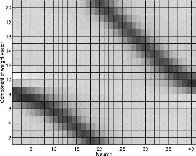
Figure 4.7:
The weight vectors of the network. The grayish colour corresponds
to zero value. The darker colours are positive values and lighter
colour are negative. Most components in the weight vectors are
very close to zero. Each neuron has learned to represent the
position of a single ``fly''.
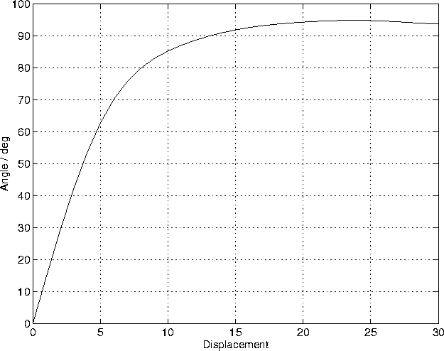
Figure 4.8:
The average angle between weight vectors as a function of their
distance in the 1-dimensional map.
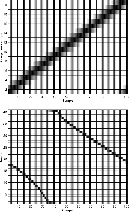
Figure 4.9:
The outputs of the map (at the bottom) for sample inputs (at the
top). White colour corresponds to zero and dark colours to
positive values.
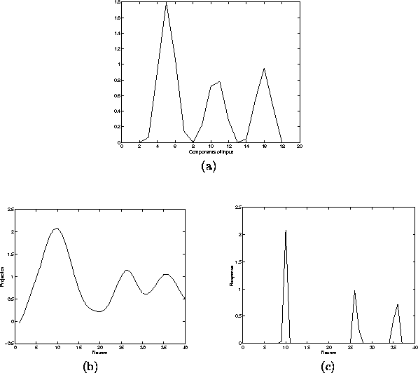
Figure 4.10:
A sample from the training set (a), the projections of the neurons
(b) and the final outputs after winning strength assignment (c).