Next the algorithm was tested with natural data. A sheet of
hand-written text was digitised with 100 dpi resolution. The samples
were obtained by taking small 16 by 16 pixels square areas corresponding to
4mm by 4mm area in the original text. In figure 4.11 (a)
there are 100 samples from the image. In the sample vectors,
background colour of the sheet was coded by zero and the text was
coded with positive values. A 2-dimensional map was adapted using
parameters in table 4.2. Parameters ![]() and
and
![]() were held constant throughout the learning.
Figure 4.11 (b) shows the weight vectors of the resulting
map. Each neuron seems to be sensitive to a dot of ink at a localised
part of the sample. It is also evident that the finite sampling area has
caused the distribution of the neurons to be far from uniform. The
neurons which are sensitive to ink at the edge of the sample are much
more localised than the neurons which are sensitive to ink at the
centre of the sample. This happens probably because there are quite
many samples where only a small part of a letter is visible at the
edge of the sample.
were held constant throughout the learning.
Figure 4.11 (b) shows the weight vectors of the resulting
map. Each neuron seems to be sensitive to a dot of ink at a localised
part of the sample. It is also evident that the finite sampling area has
caused the distribution of the neurons to be far from uniform. The
neurons which are sensitive to ink at the edge of the sample are much
more localised than the neurons which are sensitive to ink at the
centre of the sample. This happens probably because there are quite
many samples where only a small part of a letter is visible at the
edge of the sample.
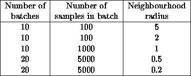
Table 4.2:
Parameters in the test runs with 100 neuron maps and natural data.
In order to decrease the effect of the finite sampling area, the samples were weighted with a Gaussian function, whose full width at half maximum was the width of the sample, i.e., the weights at the middle of the borders of a sample were 1/2. All parameters were the same as in the previous test. Figure 4.12 shows some of the samples and the resulting map. The centre of the sample received more neurons to represent it. Some neurons have elongated dots in their weight vectors. This means that these neurons are sensitive to location as well as orientation.
Next the effect of increasing the number of neurons was tested. The data was the same as in the previous test but the number of neurons was increased to 400. The parameters used in the training are shown in table 4.3. The resulting map is shown in figure 4.13. Due to the larger number of neurons there is more competition and the neurons become more specialised. The majority of the neurons are sensitive to both location and orientation.
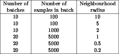
Table 4.3:
Parameters in the test run with 400 neuron map and natural data.
Figure 4.14 shows the linear reconstructions of the sample images from the outputs of the maps. The reconstructions have been computed using equation 3.8. The acuity of the reconstructions based on the map with 400 neurons is naturally better than with 100 neurons. It should be noted that equation 3.8 does not give the exact reconstruction of the inputs, but nevertheless it can be used to give an idea about the amount of information in the outputs of the network. Also, the only goal of the algorithm is not to find optimal representation with respect to reconstruction error, which could be minimised using dense coding. The outputs are also required to be sparse, which has several other advantages over dense coding.
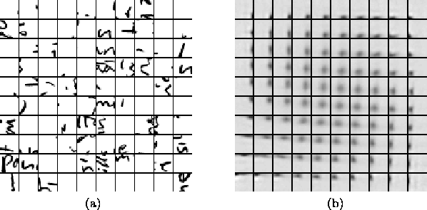
Figure:
100 samples from hand-written text (a). The text has been
digitised with 100 dpi resolution, and each sample has 16 by 16
pixels corresponding to 4mm by 4mm area. White colour corresponds
to zero and dark colours to positive values. A 2-dimensional map
with 100 neurons (b) has learned to represent the samples. Due to
the fairly small area in the samples the distribution of the
filters is far from uniform.
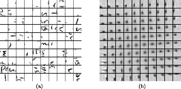
Figure:
100 samples from hand-written text (a). The samples are otherwise
similar to those in figure 4.11 (a), but in order to
decrease the effect of the finite sampling area they have been
weighted with a Gaussian function, whose full width at half maximum has
been the width of the sample, i.e., the weights at the middle of
the borders of a sample have been 1/2. A 2-dimensional map with
100 neurons (b) has learned to represent the samples. The
distribution of the filters is more uniform than in
figure 4.11 (b).
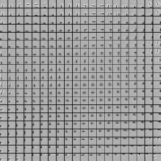
Figure:
A 2-dimensional map with 400 neurons has learned samples taken
from hand-written text. The samples have been weighted with a
Gaussian function (see figure 4.12 (a)).
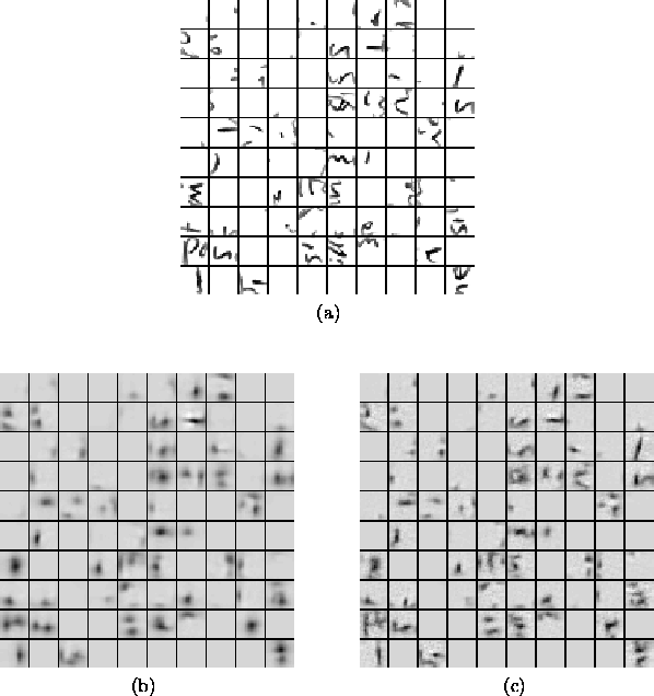
Figure:
100 samples (a) have been linerly reconstructed from the outputs
of a map with 100 neurons (b) (the map in figure 4.12)
and 400 neurons (c) (the map in figure 4.13). The
reconstructions give an idea about the amount of information in
the outputs.