We shall now summarise the algorithm. Figure 3.6
schematically shows the structure of the network. The network has a
layer of neurons, which compute projections p of the input
![]() in the direction of their weight vectors
in the direction of their weight vectors ![]() .
.
The weight vectors are normalised to unity.
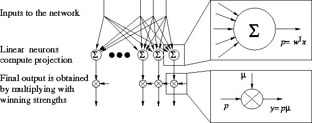
Figure 3.6:
The network has a layer of linear neurons and a mechanism which
assings winning strengths ![]() for each neuron.
for each neuron.
The efficiency of the algorithm is based on selecting for each input a
set of winners. The selection is based on winning ratios ![]() which
are defined in equation 3.6.
which
are defined in equation 3.6.
The ratios are combined according to equation 3.7, which
has to be solved numerically since the preliminary winning strengths
![]() appear in both sides of the equation. On the other hand, the
computation needs to be done for the set of winners only. The
preliminary winning strengths
appear in both sides of the equation. On the other hand, the
computation needs to be done for the set of winners only. The
preliminary winning strengths ![]() have been derived with the
following competition mechanism in mind: the stronger is the
correlation
have been derived with the
following competition mechanism in mind: the stronger is the
correlation ![]() between the weight vectors of neurons i and j
the stronger is the competition between them, and if
between the weight vectors of neurons i and j
the stronger is the competition between them, and if ![]() there is no mutual competition between neurons i and j.
there is no mutual competition between neurons i and j.
Equations 3.10, 3.11 and 3.12 are used to
compute the final winning strengths ![]() from the preliminary
winning strengths
from the preliminary
winning strengths ![]() . The final outputs
. The final outputs ![]() are obtained by
multiplying the projections with the winning strengths.
are obtained by
multiplying the projections with the winning strengths.
These equations have been chosen so that if we use the following reconstruction mapping for the input
![]()
then the reconstruction error is close to minimum.
The learning rule for the network is a combination of minimising the
reconstruction error and using neighbourhoods. It is advisable to use
the batch version of the learning rule (equation 3.18),
because the computation of correlations between the weight vectors
( ![]() ) is quite a heavy operation.
) is quite a heavy operation.