Natural Conjugate Gradient

Like with natural gradient ascent, it is often necessary to make certain simplifying assumptions to keep the iteration simple and efficient. In this paper, geodesics are approximated with (Euclidean) straight lines. This also means that parallel transport cannot be used, and vector operations between vectors from two different tangent spaces are performed in the Euclidean sense, i.e. assuming that the parallel transport between two points close to each other on the manifold can be approximated by the identity mapping. This approximative algorithm is called the natural conjugate gradient (NCG). A similar algorithm was applied to MLP network training by González and Dorronsoro (2006).

For small step sizes and geometries which are locally close to Euclidean these assumptions still retain many of the benefits of original algorithm while greatly simplifying the computations. Edelman et al. (1998) showed that near the solution Riemannian conjugate gradient method differs from the flat space version of conjugate gradient only by third order terms, and therefore both algorithms converge quadratically near the optimum.

The search direction for the natural conjugate gradient method is given by

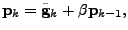$$\mathbf{p}_k = \tilde{\mathbf{g}}_k+\beta \mathbf{p}_{k-1},$$ (20)

and the Polak-Ribiére formula is given by

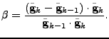$$\beta=\frac{(\tilde{\mathbf{g}}_k - \tilde{\mathbf{g}}_{k-1}) \cdot \tilde{\mathbf{g}}_k} {\tilde{\mathbf{g}}_{k-1} \cdot \tilde{\mathbf{g}}_k}.$$ (21)