NORMAL DISTRIBUTION

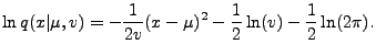
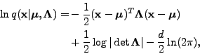
For the univariate Gaussian distribution parameterized by mean and variance $N(x;\;\mu,v)$, we have

$$\ln q(x \vert \mu,v) = - \frac{1}{2v}(x - \mu)^2 -\frac{1}{2}\ln(v)-\frac{1}{2}\ln(2\pi).$$ (7)

Further,

$$E \left\{ -\frac{\partial^2 \ln q(x \vert \mu,v )}{\partial \mu \partial \mu} \right\} = \frac{1}{v},$$ (8)

$$E \left\{ -\frac{\partial^2 \ln q(x \vert \mu,v)}{\partial v \partial \mu} \right\} = 0, \mathrm{~and}$$ (9)

$$E \left\{ -\frac{\partial^2 \ln q(x \vert \mu,v)}{\partial v \partial v} \right\} = \frac{1}{2 v^2}.$$ (10)

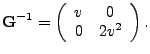
The resulting Fisher information matrix is diagonal and its inverse is given simply by

$$\mathbf{G}^{-1} = \left( \begin{array}{cc} v & 0 \\ 0 & 2v^2 \end{array} \right) .$$ (11)

In the case of univariate Gaussian distribution, natural gradient has a rather straightforward intuitive interpretation as seen in Figure 1. Compared to conventional gradient, natural gradient compensates for the fact that changing the parameters of a Gaussian with small variance has much more pronounced effects than when the variance is large. The differences between the gradient and the natural gradient are illustrated in Figure 2 with a simple example.

Figure: The absolute change in the mean of the Gaussian in figures (a) and (b) and the absolute change in the variance of the Gaussian in figures (c) and (d) is the same. However, the relative effect is much larger when the variance is small as in figures (a) and (c) compared to the case when the variance is high as in figures (b) and (d) (Valpola, 2000).

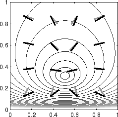
Figure: The contours show an objective function of the mean (horizontal axis) and the variance (vertical axis) of a Gaussian model. Gradient (gray line) and natural gradient (black line) are plotted at 16 different points.

For the multivariate Gaussian distribution parameterized by mean and precision $N(\mathbf{x};\;\boldsymbol{\mu},\boldsymbol{\Lambda})$, we have

$$\begin{split}\ln q(\mathbf{x}\vert \boldsymbol{\mu},\boldsymb... ...et \boldsymbol{\Lambda}\vert -\frac{d}{2}\ln(2\pi), \end{split}$$ (12)

where $d$ is the dimension of $\mathbf{x}$. Rather straightforward differentiation yields

$$E \left\{ -\frac{\partial^2 \ln q(\mathbf{x}\vert \boldsymbol{\mu... ...ymbol{\Lambda})}{\partial \boldsymbol{\mu}\partial \boldsymbol{\mu}^T} \right\} = \boldsymbol{\Lambda},$$ (13)

$$E \left\{ -\frac{\partial^2 \ln q(\mathbf{x}\vert \boldsymbol{\mu... ...bol{\Lambda})}{\partial \boldsymbol{\mu}\partial \boldsymbol{\Lambda}} \right\} = 0,$$ (14)

$$E \left\{ -\frac{\partial^2 \ln q(\mathbf{x}\vert \boldsymbol{\mu... ...\Lambda})}{\partial \boldsymbol{\Lambda}\partial \boldsymbol{\Lambda}} \right\} = \frac{1}{2} \boldsymbol{\Lambda}^{-1} \otimes \boldsymbol{\Lambda}^{-1},$$ (15)

where $\otimes$ is the direct product, also known as the Kronecker product. Because the cross term is zero, the resulting full Fisher information matrix is block diagonal and can be inverted simply by

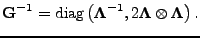$$\mathbf{G}^{-1} = \mathrm{diag}\left(\boldsymbol{\Lambda}^{-1}, 2 \boldsymbol{\Lambda}\otimes \boldsymbol{\Lambda}\right).$$ (16)

This result for the precision may not be very useful in practice, as the approximations used in most applications have a more restricted form such as a Gaussian with a factor analysis covariance 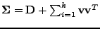$\mathbf{\Sigma} = \mathbf{D} + \sum_{i=1}^k \mathbf{v} \mathbf{v}^T$, where $\mathbf{D}$ is a diagonal matrix, or a Gaussian Markov random field.