INFORMATION GEOMETRY AND NATURAL GRADIENT

Let $\mathcal{F}(\boldsymbol{\xi})$ be a scalar function defined on the manifold $S=\{ \boldsymbol{\xi}\in \mathbf{R}^n \}$. If $S$ is a Euclidean space and the coordinate system $\boldsymbol{\xi}$ is orthonormal, the length of a small incremental vector $\mathbf{w}$ is given by

$$\vert\mathbf{w}\vert^2=\sum_{i=1}^n w_i^2,$$ (1)

where $w_i$ is the $i$th component of the vector $\mathbf{w}$. The direction of steepest ascent, i.e. the direction that maximizes $\mathcal{F}(\boldsymbol{\xi}+ \mathbf{w})$ under the constraint $\vert\mathbf{w}\vert^2=\epsilon^2$ for a sufficiently small constant $\epsilon$, is given by the gradient $\nabla \mathcal{F}(\boldsymbol{\xi})$.

If the space $S$ is a curved manifold, there is no orthonormal coordinate system and the the length of a vector $\mathbf{w}$ differs from the value given by Eq. (1). Riemannian manifolds are an important class of curved manifolds, where the length is given by the positive quadratic form

$$\vert\mathbf{w}\vert^2=\sum_{i,j} g_{ij}(\boldsymbol{\xi}) w_i w_j.$$ (2)

The $n \times n$ matrix $\mathbf{G}(\boldsymbol{\xi})=(g_{ij}(\boldsymbol{\xi}))$ is called the Riemannian metric tensor and it may depend on the point of origin $\boldsymbol{\xi}$. On a Riemannian manifold, the direction of steepest ascent is given by the natural gradient (Amari, 1998)

$$\tilde{\nabla} \mathcal{F}(\boldsymbol{\xi}) = \mathbf{G}^{-1}(\boldsymbol{\xi}) \nabla \mathcal{F}(\boldsymbol{\xi}).$$ (3)

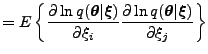
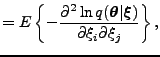
For the space of probability distributions $q(\boldsymbol{\theta}\vert \boldsymbol{\xi})$, the most common Riemannian metric tensor is given by the Fisher information (Amari, 1985)

$$I_{ij}(\boldsymbol{\xi}) = g_{ij}(\boldsymbol{\xi}) = E \left\{ \frac{\partial \ln q(\boldsymbol{\theta}\vert \boldsy... ...ial \ln q(\boldsymbol{\theta}\vert \boldsymbol{\xi})} {\partial \xi_j} \right\}$$ (4)

$$= E \left\{ -\frac{\partial^2 \ln q(\boldsymbol{\theta}\vert \boldsymbol{\xi})} {\partial \xi_i \partial \xi_j} \right\},$$

where the last equality is valid given certain regularity conditions (Murray and Rice, 1993).