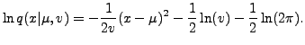
For the univariate Gaussian distribution parametrized by mean and variance
![]() , we have
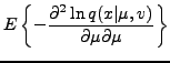
, we have
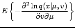
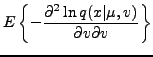
Furthermore,
In the case of univariate Gaussian distribution, natural gradient for the mean has a rather straightforward intuitive interpretation, which is illustrated in Figure 1 (left). Compared to conventional gradient, natural gradient compensates for the fact that changing the parameters of a Gaussian with small variance has much more pronounced effects than when the variance is large.
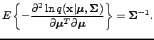
In case of multivariate Gaussian distribution, the elements of the Fisher information matrix corresponding to the mean are simply