Next: Subspace Learning Algorithm
Up: Principal Component Analysis for
Previous: Introduction
Assume that we have 
 -dimensional data vectors
 , which form the
  data matrix
 =
=
![$ [{\bf x}_1,{\bf x}_2,\ldots,{\bf x}_n]$](img8.png) . The matrix
is
decomposed into
. The matrix
is
decomposed into
 , where
 is a
is a  matrix,
 is a
is a  matrix and
 . Principal
subspace methods [6,4] find such
and
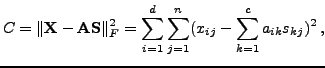
that the reconstruction error
. Principal
subspace methods [6,4] find such
and
that the reconstruction error
is minimized. Typically the row-wise mean is removed from
as a
preprocessing step. Without any further constraints, there exist
infinitely many ways to perform such a decomposition. PCA constraints
the solution by further requiring that the column vectors of
are
of unit norm and mutually orthogonal and the row vectors of
are
also mutually orthogonal
[3,4,2,5].
There are many ways to solve PCA
[6,4,2]. We will concentrate on the
subspace learning algorithm that can be easily adapted for the case of
missing values and further extended.
Subsections
Tapani Raiko
2007-07-16