![[*]](cross_ref_motif.gif) . The data points
correspond to different time indices t. The second layer, like the
first one, has two dimensions: the first corresponds to the direction
left and the second to the up right from the bias
. The data points
correspond to different time indices t. The second layer, like the
first one, has two dimensions: the first corresponds to the direction
left and the second to the up right from the bias
A simple example illustrates the long definition of HNFA+VM. Even though the learning algorithm is not yet presented, the resulting model taught with two dimensional toy data is discussed here. As is typical for nonlinear problems, the algorithm can only find a local optimum that depends on the initialisation. A local optimum of a good model is usually better than a global optimum of a bad one. In this case, the found network is not optimal but perhaps instructive. It is explained from bottom up.
HNFA+VM with three layers is taught with the two-dimensional
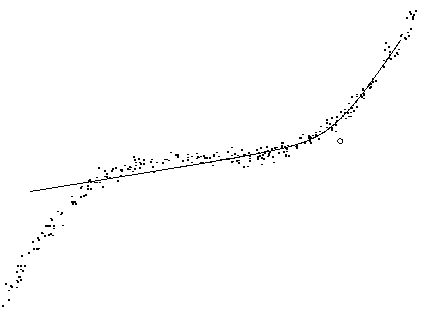
data shown by dots in Figure ![[*]](cross_ref_motif.gif) . The data points
correspond to different time indices t. The second layer, like the
first one, has two dimensions: the first corresponds to the direction
left and the second to the up right from the bias
. The data points
correspond to different time indices t. The second layer, like the
first one, has two dimensions: the first corresponds to the direction
left and the second to the up right from the bias
![]() marked with a circle. The single neuron in the third layer affects
the neurons on the second layer and through them the data
reconstructions. Possible values of the source s3,1 form a curve
in the data space.
marked with a circle. The single neuron in the third layer affects
the neurons on the second layer and through them the data
reconstructions. Possible values of the source s3,1 form a curve
in the data space.
 |
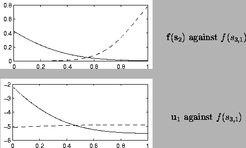
Figure ![[*]](cross_ref_motif.gif) illustrates the effects of the neuron in
the third layer in more detail. At one end of its spectrum, it
activates the first neuron in the second layer and at the other end,
the second neuron. In the middle, both neurons are affected and the
curvature of the data, is modelled. Most of the weights
B to the variance neurons are close to zero, but the
connection B1,2,1 from the first dimension of the second layer to
the vertical dimension of the data plane is very different. The effect
can be seen in the lower part of the same figure.
illustrates the effects of the neuron in
the third layer in more detail. At one end of its spectrum, it
activates the first neuron in the second layer and at the other end,
the second neuron. In the middle, both neurons are affected and the
curvature of the data, is modelled. Most of the weights
B to the variance neurons are close to zero, but the
connection B1,2,1 from the first dimension of the second layer to
the vertical dimension of the data plane is very different. The effect
can be seen in the lower part of the same figure.
 |
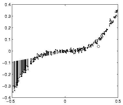
Each data point is connected to the mean of its reconstruction
ms1 in Figure ![[*]](cross_ref_motif.gif) . The reconstructions
are near the actual data points, except in the far left.
In that region, the vertical variance neuron is activated. This
explains why the reconstructions are allowed to be vertically
inaccurate there.
. The reconstructions
are near the actual data points, except in the far left.
In that region, the vertical variance neuron is activated. This
explains why the reconstructions are allowed to be vertically
inaccurate there.
 |
The third layer has one source s3,1 and the corresponding variance neuron u3,1. The prior sdistribution of the source s3,1 is depicted in
Figure ![[*]](cross_ref_motif.gif) .
The
distribution is very close to a Gaussian, since the corresponding
variance neuron happens to be inactive. Otherwise it would have been
symmetric but super-Gaussian as explained in
Section
.
The
distribution is very close to a Gaussian, since the corresponding
variance neuron happens to be inactive. Otherwise it would have been
symmetric but super-Gaussian as explained in
Section ![[*]](cross_ref_motif.gif) . The nonlinearity distorts the distribution
such that the other end has a longer tail.
. The nonlinearity distorts the distribution
such that the other end has a longer tail.
 |
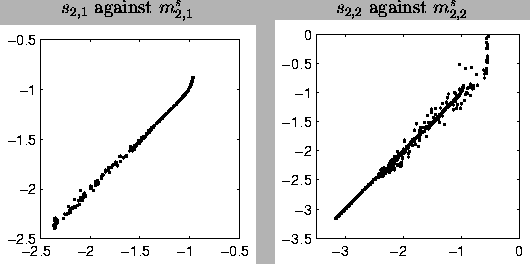
The behaviour of the model can be compared to that of a multilayer
perceptron (MLP) network. In the MLP network, the sources of the
second layer would have been computational hidden units and therefore
their signals would have been functions of the third layer signal. In
the HNFA+VM case the difference of input and output signals of the
middle layer can be seen in Figure ![[*]](cross_ref_motif.gif) .
The values are somewhat close to the diagonal line which means that
the second layer behaves somewhat like a computational layer. The
variation from the diagonal corresponds to the fact that the
reconstructions in Figure
.
The values are somewhat close to the diagonal line which means that
the second layer behaves somewhat like a computational layer. The
variation from the diagonal corresponds to the fact that the
reconstructions in Figure ![[*]](cross_ref_motif.gif) are not exactly on
the curve. The variance neurons have no counterparts in the MLP
framework.
are not exactly on
the curve. The variance neurons have no counterparts in the MLP
framework.
 |
With another initialisation the presumably globally optimal solution
shown in Figure ![[*]](cross_ref_motif.gif) , was found. A third source in the
second layer took care of the left part and all the reconstructions
became relatively accurate. Variance neurons were of no use in this
solution. The existence of local optimum in a simple problem like this
suggests that it is far from trivial to design a good learning
procedure and therefore the entire Chapter
, was found. A third source in the
second layer took care of the left part and all the reconstructions
became relatively accurate. Variance neurons were of no use in this
solution. The existence of local optimum in a simple problem like this
suggests that it is far from trivial to design a good learning
procedure and therefore the entire Chapter ![[*]](cross_ref_motif.gif) is dedicated
to it.
is dedicated
to it.