Sparse Coding

In many of the described models, the observations are reconstructed as a weighted sum of model vectors. In vector quantisation [1], only one of the model vectors is active at a time, which means that all but one of the weights are zero. This is called local coding. There has to be lots of model vectors to get a reasonable accuracy. In basic factor analysis, the factors have a Gaussian distribution and therefore most of them can be active or nonzero at a time. This is called global coding. Sparse coding fits in between these two extremes; Each observation is reconstructed using just a few active units out of a larger collection. Biological evidence suggests [14] that the human brain uses sparse coding. It is said to have benefits like good representational capacity, fast learning, good generalisation and tolerance to faults and damage.

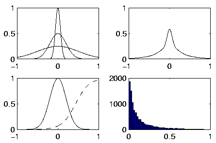
Sparsity implies that the distribution of a source has a high peak, but the variation can still be broad. The peak corresponds to the inactivity and therefore it is typically at zero. Kurtosis is one measure of peakedness. It is defined as

$$\text{kurt}(s) = E\{s^4\}-3\left[E\{s^2\}\right]^2,$$ (2.17)

if s is assumed to have zero mean. For Gaussian distributions, the kurtosis is zero and for peaked and heavy tailed, it is positive. ICA can be carried out by maximising the absolute values of the kurtosis which means that it can promote sparsity.

Most of the probability density functions in this thesis are Gaussian. However, by varying the variance or using a nonlinearity with a flat part as in Figure , a peaked distribution can be obtained. Beale showed [4] that by varying the variance of a symmetrical distribution, the kurtosis always increases. Because of the biological and experimental motivation to use sparse coding, it is made sure in Chapter  that the model is rich enough to use it.

  

Figure: Two ways to obtain a supergaussian distribution from a Gaussian one. Top: The mean of three Gaussians with different variances is taken. Bottom: a Gaussian is fed through a nonlinearity marked with the dashed curve. The resulting distributions are shown on the right hand side.