

Next: Hierarchical Prior for the
Up: Formulation of the Model
Previous: Formulation of the Model
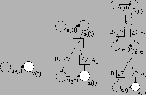
Figure ![[*]](cross_ref_motif.gif) shows the structure for
hierarchical nonlinear factor analysis with variance modelling
(HNFA+VM). It utilises variance neurons and nonlinearities in
building a hierarchical model for both the means and variances.
Without the variance neurons the model would correspond to a
multi-layer perceptron with latent variables as hidden neurons. Note
that computational nodes as hidden neurons would result in multiple
paths from upper layer latent variables to the observations. This
type of structure was used in [43] and it has a quadratic
as opposed to linear computational complexity.
shows the structure for
hierarchical nonlinear factor analysis with variance modelling
(HNFA+VM). It utilises variance neurons and nonlinearities in
building a hierarchical model for both the means and variances.
Without the variance neurons the model would correspond to a
multi-layer perceptron with latent variables as hidden neurons. Note
that computational nodes as hidden neurons would result in multiple
paths from upper layer latent variables to the observations. This
type of structure was used in [43] and it has a quadratic
as opposed to linear computational complexity.
Figure:
HNFA+VM model can be built up in stages. Left: A variance neuron is
attached to each Gaussian observation node. The nodes represent
vectors. Middle: A layer of sources with variance neurons attached
to them is added. The nodes next to the weight matrices
A1 and
B1 represent affine transformations
including a bias term. Right: Another layer is added. The size of
the layers may vary. More layers can be added in the same
manner. Note that some parameters are left out of the picture for
clarity.
 |
The exact formulation of HNFA+VM is as follows. The observed
data matrix
X has T observations of n1 dimensions.
X is named
s1(t) for notational simplicity
![\begin{displaymath}\boldsymbol{X}= \left[\mathbf{s}_{1}(1),\mathbf{s}_{1}(2),\dots,\mathbf{s}_{1}(T)\right],
\end{displaymath}](img189.gif) |
(5.1) |
where
 corresponds to different observations
and the subscript 1 corresponds to the first layer.
On each layer i, there are ni sources assembled to a vector
si. The dimensions of the vectors are marked with
si,k,
 .
The sources on upper layers i>1are mapped through a Gaussian nonlinearity
| f(si(t)) |
= |
![$\displaystyle \left[ \begin{array}{c}
\exp(-s_{i,1}(t)^2) \\
\exp(-s_{i,2}(t)^2) \\
\vdots \\
\exp(-s_{i,n_i}(t)^2) \end{array} \right].$](img191.gif) |
(5.2) |
The connection downwards after the nonlinearity is done using the
affine mappings
| mis(t) |
= |
 |
(5.3) |
| miu(t) |
= |
 |
(5.4) |
where n is the number of layers.
Each source si,k has a corresponding variance neurons
ui,k. The signals
mis(t) and
miu(t)are used as prior means for them
The prior variance of source vector
si(t) is the
corresponding variance source vector
ui,k(t) and the prior
variance of variance sources is a parameter vector
 .
.


Next: Hierarchical Prior for the
Up: Formulation of the Model
Previous: Formulation of the Model
Tapani Raiko
2001-12-10
![[*]](cross_ref_motif.gif) shows the structure for
hierarchical nonlinear factor analysis with variance modelling
(HNFA+VM). It utilises variance neurons and nonlinearities in
building a hierarchical model for both the means and variances.
Without the variance neurons the model would correspond to a
multi-layer perceptron with latent variables as hidden neurons. Note
that computational nodes as hidden neurons would result in multiple
paths from upper layer latent variables to the observations. This
type of structure was used in [43] and it has a quadratic
as opposed to linear computational complexity.
shows the structure for
hierarchical nonlinear factor analysis with variance modelling
(HNFA+VM). It utilises variance neurons and nonlinearities in
building a hierarchical model for both the means and variances.
Without the variance neurons the model would correspond to a
multi-layer perceptron with latent variables as hidden neurons. Note
that computational nodes as hidden neurons would result in multiple
paths from upper layer latent variables to the observations. This
type of structure was used in [43] and it has a quadratic
as opposed to linear computational complexity.

![$\displaystyle \left[ \begin{array}{c}
\exp(-s_{i,1}(t)^2) \\
\exp(-s_{i,2}(t)^2) \\
\vdots \\
\exp(-s_{i,n_i}(t)^2) \end{array} \right].$](img191.gif)

