Factor Analysis

The basic approach is simply called factor analysis [22,38] (FA). The data x(t) is thought to have been generated from factors s(t) through a linear mapping A using the formula

 

x(t) = As(t) + n(t), (2.1)

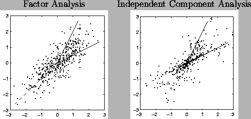
where n(t) is noise or reconstruction error vector. The vectors As(t) are called the reconstructions. Typically the dimensionality of the factors is smaller than that of the data. Factors and noise are assumed to have a Gaussian distribution. Figure  shows a two dimensional example. Factor analysis can be seen as trying to fit a Gaussian distribution to the data points.

  

Figure: Left: Factor Analysis. The image has been generated by mixing two Gaussian factors with a matrix visualised with the solid lines. In factor analysis, the rotation is not fixed, but principal component analysis selects the orientation with orthogonal axis shown with the dash lines. Right: When the factors have non-Gaussian distributions the rotation is fixed and can be found using independent component analysis.

Equation  does not fix the matrix A, since there is a group of rotations that yield identical observation distributions. Several criteria have been suggested for determining the rotation. One is called the parsimony, which roughly means that most of the values in A are close to zero. Others include independency of the factors and discarding the assumption of Gaussian distribution of them and instead maximising the nongaussianity. These have led to independent component analysis [31,35] (ICA) that is described below.