Nonstationary variance

Figure 3: Left: The Gaussian variable $s(t)$ has a a constant variance $\exp(-v)$ and mean $m$. Right: A variance source is added for providing a non-constant variance input $u(t)$ to the output (source) signal $s(t)$. The variance source $u(t)$ has a prior mean $v$ and prior variance $\exp(-w)$.

Figure 4: The distribution of $s(t)$ is plotted when $s(t)\sim \mathcal N(0,\exp [-u(t)])$ and $u(t)\sim \mathcal N(0,\cdot)$. Note that when $\mathrm{Var}\left\{u(t)\right\}=0$, the distribution of $s(t)$ is Gaussian. This corresponds to the right subfigure of Fig. 3 when $m=v=0$ and $\exp(-w)=0,1,2$.

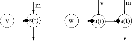
In most currently used models, only the means of Gaussian nodes have hierarchical or dynamical models. In many real-world situations the variance is not a constant either but it is more difficult to model it. For modelling the variance, too, we use the variance source Valpola04SigProc depicted schematically in Figure 3. Variance source is a regular Gaussian node whose output $u(t)$ is used as the input variance of another Gaussian node. Variance source can convert prediction of the mean into prediction of the variance, allowing to build hierarchical or dynamical models for the variance.

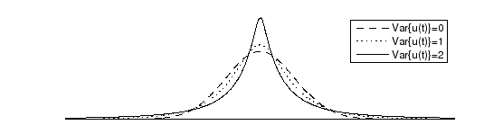
The output $s(t)$ of a Gaussian node to which the variance source is attached (see the right subfigure of Fig. 3) has in general a super-Gaussian distribution. Such a distribution is typically characterised by long tails and a high peak, and it is formally defined as having a positive value of kurtosis (see ICABook01 for a detailed discussion). This property has been proved for example in Parra00NIPS, where it is shown that a nonstationary variance (amplitude) always increases the kurtosis. The output signal $s(t)$ of the stationary Gaussian variance source depicted in the left subfigure of Fig. 3 is naturally Gaussian distributed with zero kurtosis. The variance source is useful in modelling natural signals such as speech and images which are typically super-Gaussian, and also in modelling outliers in the observations.